Synopsis

Keywords: MR Fingerprinting/Synthetic MR, MR Fingerprinting

Clinical contrasts can be generated from a 1 min 1 mm isotropic whole brain MRF scan and B0 correction improves it further. We tested this method in healthy volunteers as well as clinical populations.

Introduction

Fast multicontrast sequences are promising alternatives to conventional protocols in clinical settings as they allow for comprehensive brain assessments in just a few minutes, reducing the requirement for remaining still for a long time for patients that might struggle to do so (e.g. pediatric patients).

In this project we use MR Fingerprinting (MRF), which is a quantitative imaging method, for multi-contrast synthesis. Characterizing the tissue allows modeling of the contrast of conventional sequences. However, a complete tissue model is challenging to create manually (e.g. due to a large number of magnetization transfer related parameters), so we utilize a deep learning (DL) algorithm to generate a model from the acquired images in a temporal subspace domain to the desired contrasts. We also employ data compression and reconstruction optimization methods to reduce the reconstruction time. The pipeline we present can generate five contrasts of 1-mm isotropic resolution whole-brain images in a scan time of 1 minute and reconstruction times ranging from 5 to 15 minutes on a single GPU. A large scale clinical assessment study with over 50 patients is underway.

Methods

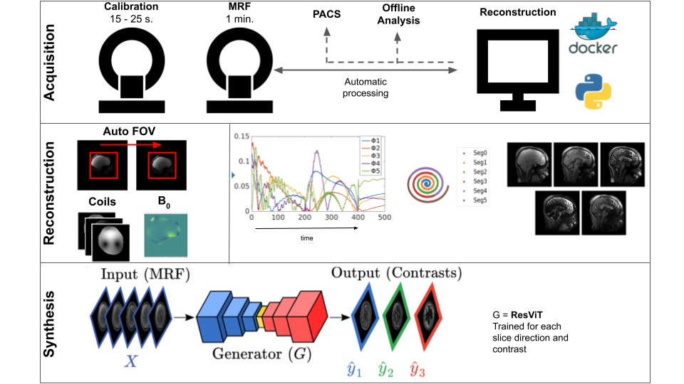
All data were acquired on a GE 3T SIGNA Premier scanner. And reconstructed using SigPy. Synthesis was performed using PyTorch. All parts of the pipeline were written in Python, and containerized using Docker. Figure 1 shows an overview of the processing pipeline.

Acquisition: The proposed pipeline consists of two sequences: (i) a 15-25 second 3D Bloch-Siegert based calibration scan (PhysiCal [1]) used to estimate coil sensitivity maps (CSM) and B0 inhomogeneities, and (ii) a multi-axis spiral projection MRF[2] sequence with 1 mm isotropic whole brain resolution. The data acquisition (without B0 correction) is modelled as: $$$b = FSΦx$$$. Here, $$$F$$$ is the non uniform Fourier transform, $$$S$$$ is the CSM and $$$Φ$$$ is a low-rank subspace that models signal evolution (see [2] for more information). $$$b$$$ denotes the acquired data and $$$x$$$ denotes the desired underlying coefficient images such that $$$Φx$$$ recovers the evolution of signal over time. $$$FSΦ$$$ will be noted $$$A$$$ henceforth.

Reconstruction: Without B0, the reconstruction is phrased as: $$$||D(Ax – b)||_2^2 + \lambda R(x)$$$. $$$D$$$ is pipe-menon density compensation and $$$R()$$$ is a regularization function, in [2] locally low rank was used and FISTA[3] was used for reconstruction. For reconstruction speed, we propose an unregularized conjugate gradient reconstruction instead. B0 inhomogeneities were accounted for by segmenting the MRF readout into $$$N$$$ discrete segments. The data within each segment is approximated to have equal amounts of phase evolution due to B0. The greater the $$$N$$$, the more accurate the model but at the cost of more intensive reconstruction. In this work, we find $$$N = 6$$$ to be suitable. Let $$$A_i$$$ denote the forward model of the ith readout segment corresponding to data segment $$$b_n$$$. The forward model is now:$$$b_n = A_i e^{i 2 \pi B_0 t_n}x$$$ for $$$n$$$ in $$$\{0, 1, .. 5\}$$$.

Synthesis: A new DL network (ResViT[4]) was used. The network was trained on individual slices in axial, coronal, and sagittal view and each target contrast separately. The target images acquired in 12 healthy subjects were T2-FLAIR, T2-Cube, T1-Cube, T1-MPRAGE, and Double Inversion Recovery (DIR) - Cube. Total scan time for the reference images was 28 minutes (with acceleration factors varying between 2 and 4). Quantitative maps were generated using standard dictionary matching.

Results

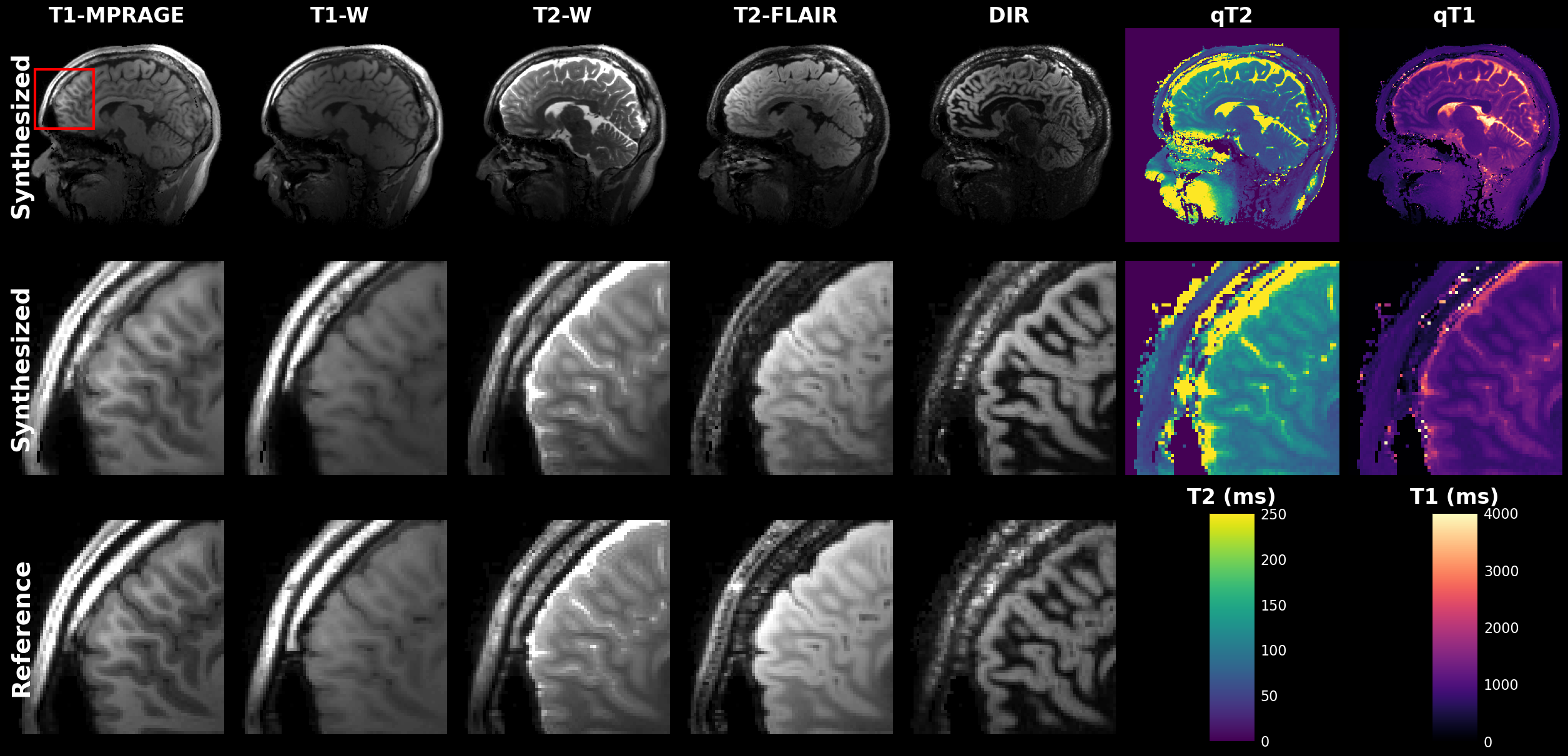
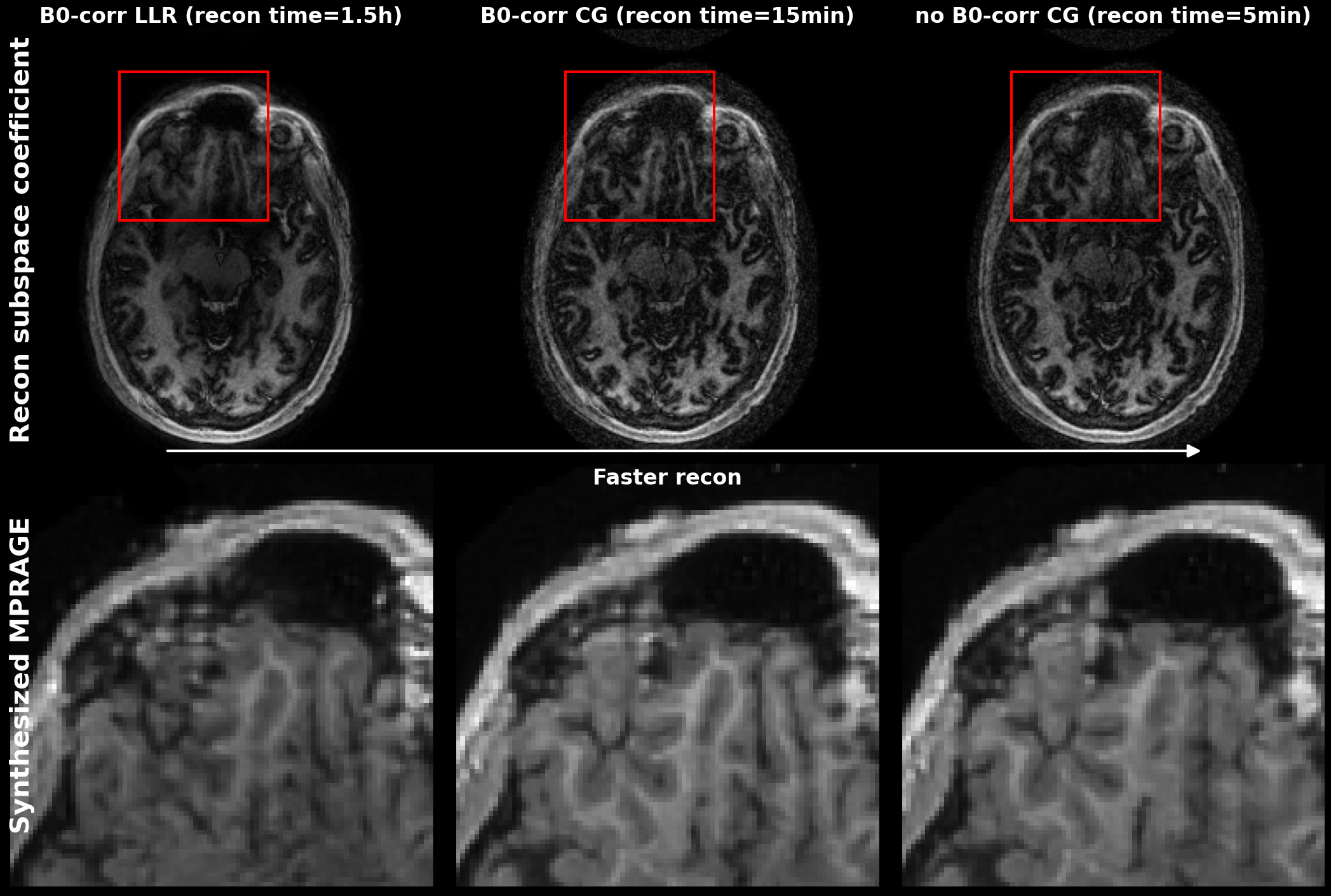
Figure 2 shows the output of a single 1min MRF scan: five synthetic contrasts as well as quantitative T2 and T1 maps. High correspondence to the reference scans were observed.

B0-correction allowed for sharper subspace coefficient maps in areas near the sinuses. The synthesis result improved for the B0 corrected inputs. However, a reference less noisy reconstruction[2], did not improve synthesis results (see Figure 3).

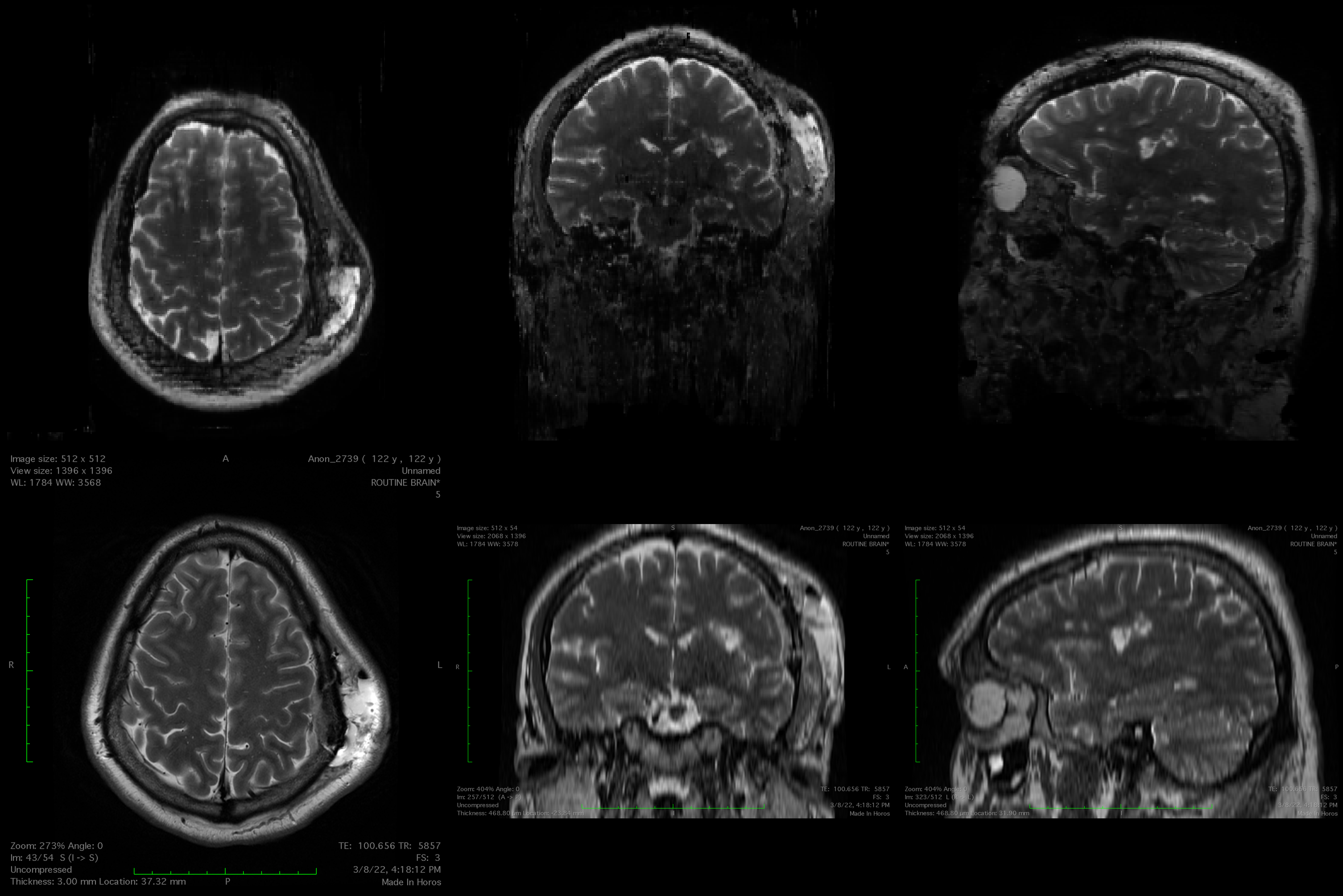
Pathologies were also visible in the synthesized images although the network had only been trained on healthy volunteer data. An example is shown in Figure 4.

Discussion and Conclusions

The results show that good synthesis can be performed with a noisy input, as the synthesis network acts as a denoiser, allowing for fast reconstruction pipelines. B0 correction improves the coefficient maps, which has a small effect on the synthesis, but can effect on the quantitative maps.

To improve this method further we can also perform B1 correction on the quantitative maps, as the PhysiCal sequence allows for B1 mapping.

As this pipeline is being clinically deployed, a study comparing the synthesized MRF with conventional clinical scans and other rapid multicontrast scans (e.g. NeuroMix[5]) is planned.

Acknowledgements

This study is supported in part by GE Healthcare research funds and NIH R01EB020613, R01MH116173, R01EB019437, U01EB025162, P41EB030006