2183
Deep learning optimization of CEST MR Fingerprinting (CEST-MRF) for Quantitative Human Brain Mapping1Medical Physics, Memorial Sloan Kettering, New York, NY, United States
Synopsis
Keywords: MR Fingerprinting/Synthetic MR, CEST & MT
CEST MR fingerprinting (CEST-MRF) enables fast quantitative relaxation and exchange mapping. The CEST-MRF signal depends on multiple acquisition and tissue parameters which makes optimization of the acquisition schedule challenging. The goal of this work is to develop a deep learning approach that uses a quantification network and a surrogate network to optimize the acquisition schedule for in vivo scans. Numerical simulations are used to characterize the optimized schedule and the benefits of optimization are demonstrated in vivo in a healthy subject. The optimized schedule can reduce scan time by 12% and provide better image quality than a randomly generated schedule.Introduction
CEST MRI, a molecular imaging technique utilizing the exchange of saturation between the mobile protons and the bulk water, was recently combined with MR fingerprinting (CEST-MRF) for fast quantitative relaxation and exchange mapping [1], [2]. However, the acquisition schedule was not optimized, which is challenging due to the signal dependance on multiple acquisition and tissue parameters. Inspired by previous work in schedule optimization on a pre-clinical scanner [3], [4], this work extends the deep learning (DL) optimization approach for in vivo scans while accounting for instrumental variations (e.g. B1 inhomogeneity). Numerical simulations are used to characterize the optimized schedule and the benefits of optimization are demonstrated in vivo in a healthy subject in comparison to a conventional acquisition schedule.Methods
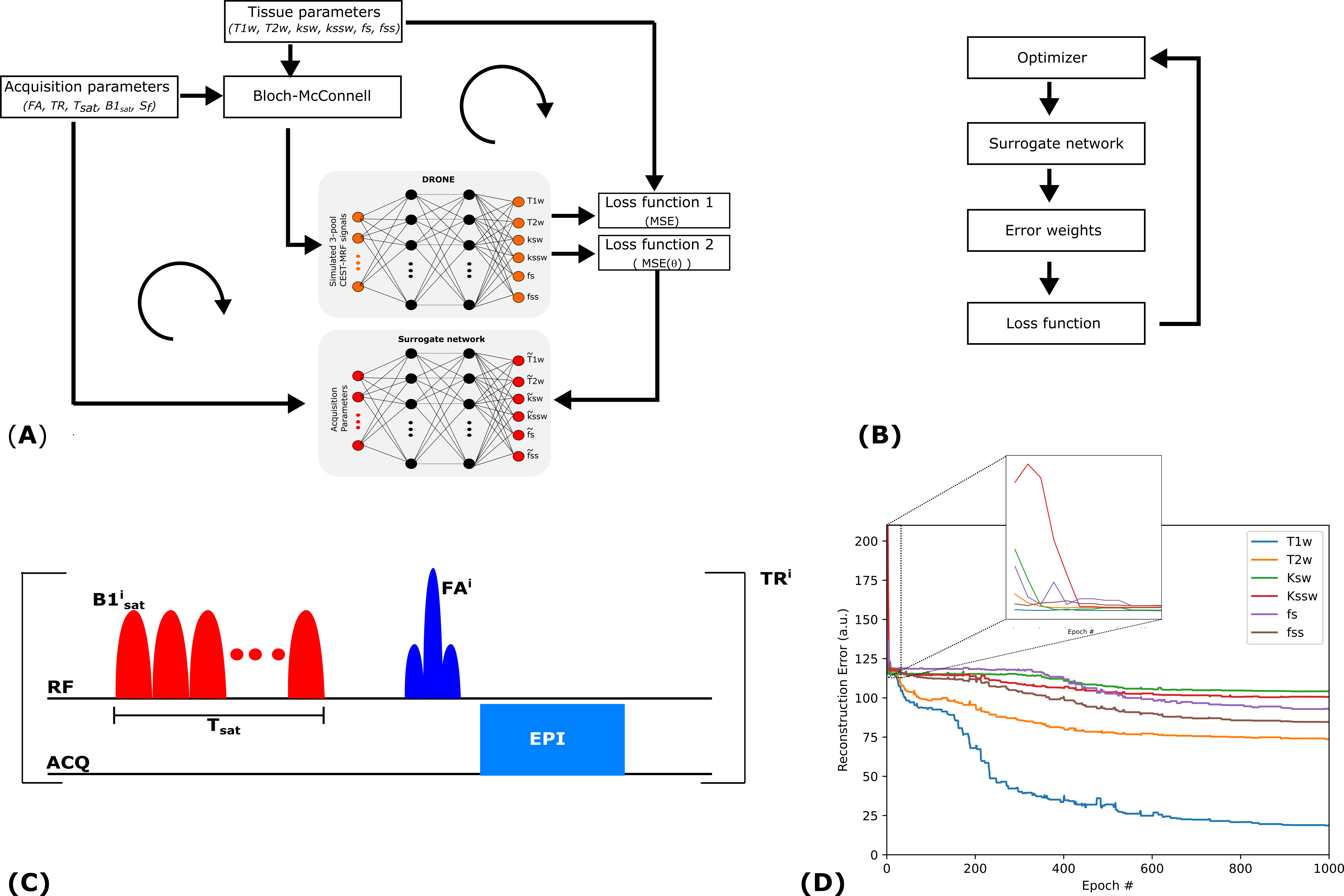
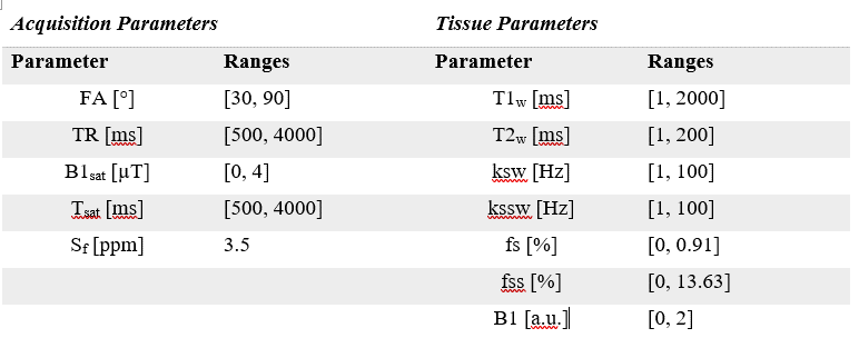
Tissue quantification network trainingFigure 1 shows an overview of the proposed method. A set of P=1000 schedules, each consisting of N=30 time-points, were sampled [5] from the acquisition parameter ranges shown in Figure 2. The saturation offset Sf was set to the amide resonance offset (3.5 ppm) whereas the other parameters were varied for each time point. For each schedule, a training dataset was defined by sampling 5000 entries from the tissue parameter ranges (Figure 2). The signal magnetizations were calculated by solving the 3-pool (water, solute, semi-solid) Bloch-McConnel equations for each set of tissue parameters. The B1 field inhomogeneity was excluded from the loss calculation to induce the network to minimize the error in the other parameters instead. A 4-layer deep reconstruction network (DRONE) [6] implemented in PyTorch was used to quantify the error in the parameter reconstruction for a given schedule. The network was trained to convergence using the ADAM optimizer [7] with a batch size of 1000, adaptive learning rate of 0.0001 and the L1 loss function.
Surrogate network definition
A second neural network was defined with the same architecture as the DRONE network but with a 150-nodes input layer corresponding to the 5 acquisition parameters for each of the 30 time-points. The training dataset for this network consisted of the P acquisition schedules and the reconstruction error vectors calculated by the tissue quantification network (Figure 1A). The network was trained for 3000 epochs with the same parameters defined above and provided a mapping between the schedule and reconstruction-error spaces.
Schedule optimization
The surrogate network permits an efficient exploration of the schedule-space (Figure 1B). To find a globally optimal schedule, 50 candidate schedules were randomly generated and used as the initialization for a pattern-search optimizer implemented in Python [8], [9]. The optimized schedule with the smallest cost was used for all subsequent experiments.
Numerical simulations
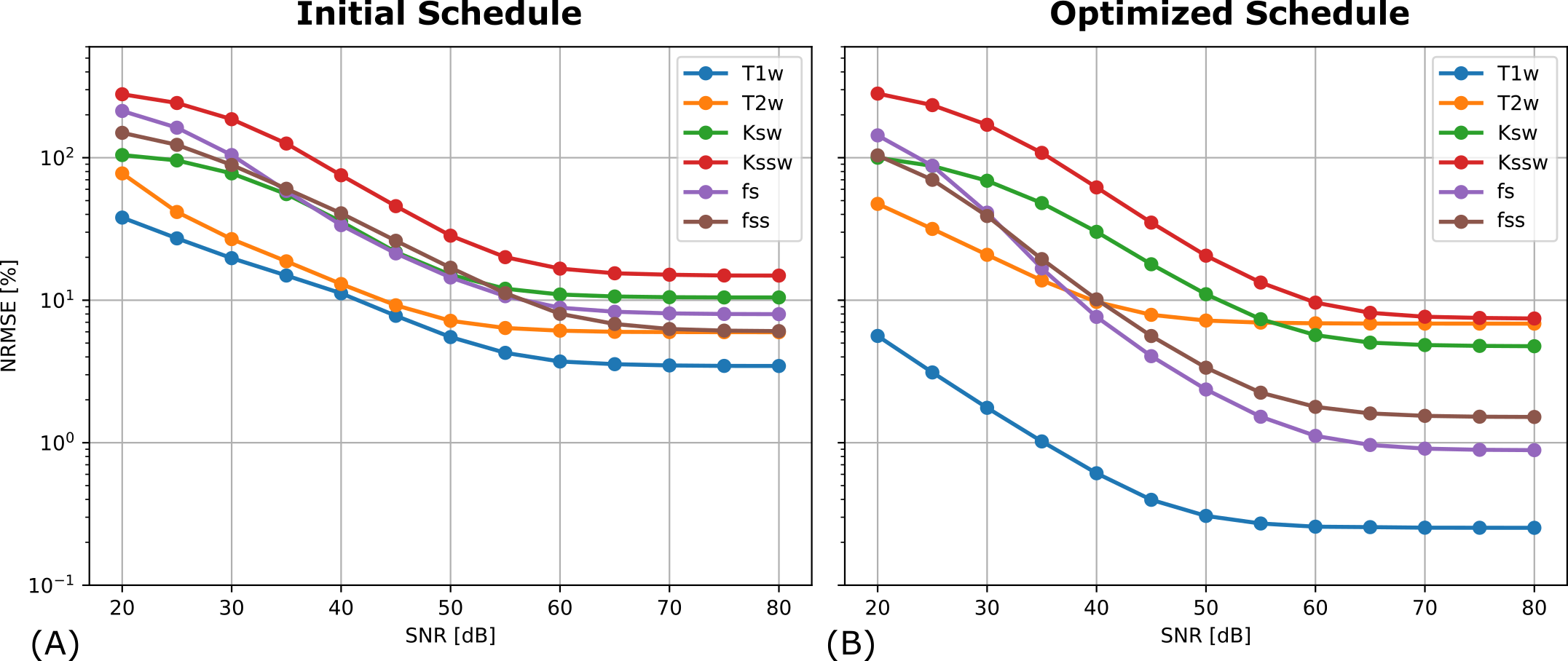
The optimized schedule was assessed in a custom modified digital phantom [10] via CEST-MRF simulation. The simulated data was reconstructed using a trained DRONE network. The normalized RMS error (NRSME) was calculated for varying levels of SNR by injecting white Gaussian noise into simulated data obtained with a conventional schedule and an optimized schedule.
In vivo comparison in a healthy subject
A healthy, 34 years old female volunteer was recruited and gave informed consent in accordance with the institutional IRB protocol. The subject was scanned on a Signa Premier 3T scanner (GE Healthcare, Waukesha, WI) with a 48-channel head receiver coil. The subject was scanned twice with the CEST-MRF sequence, first using a conventional schedule and then with the optimized schedule, with the following image acquisition parameters: matrix size/resolution/slice thickness/TE/bandwidth=192×192/1.5×1.5 mm2/5 mm/21 ms/250 kHz. The measured data from each schedule was reconstructed with a DRONE network.
Results
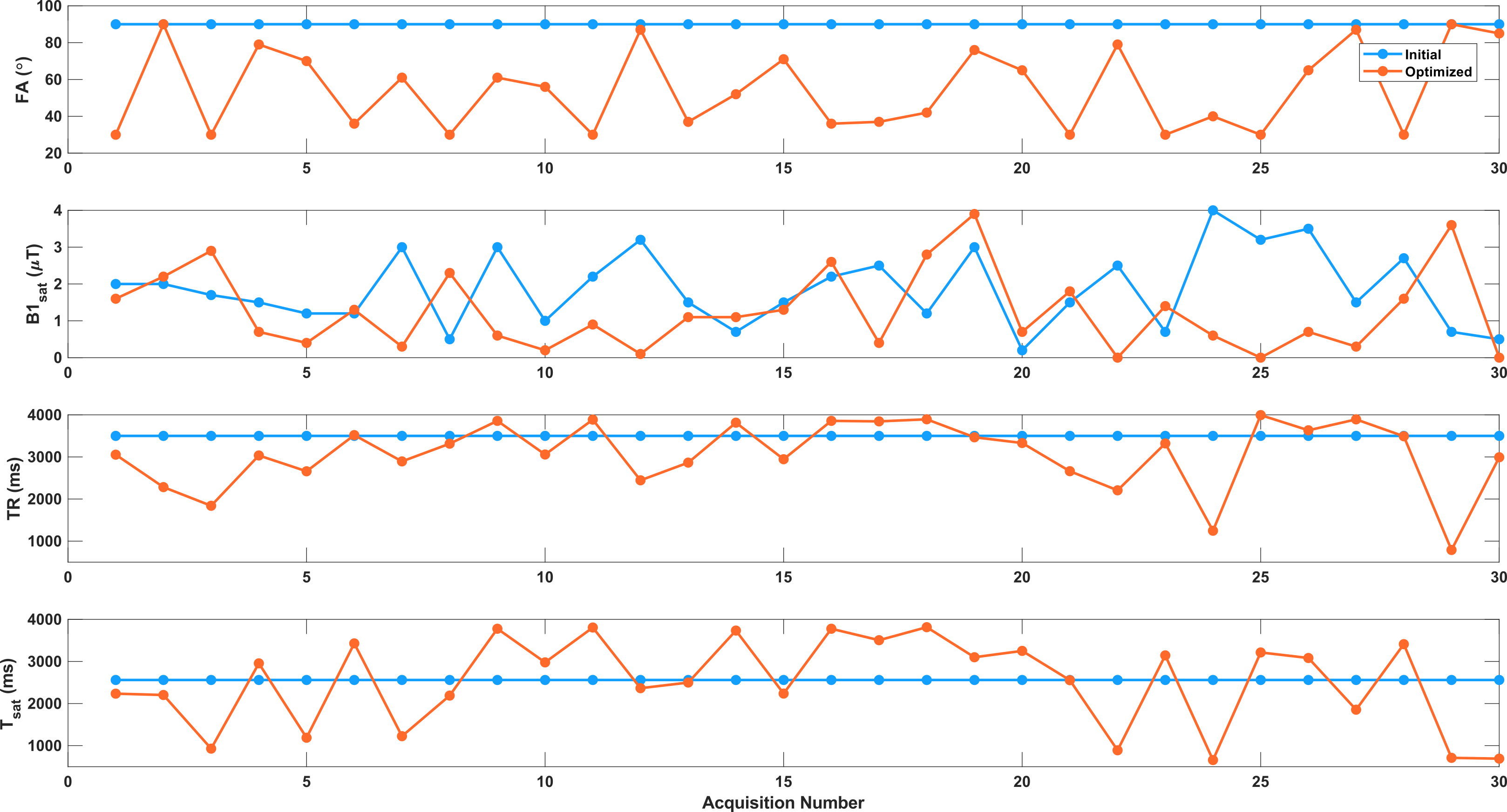
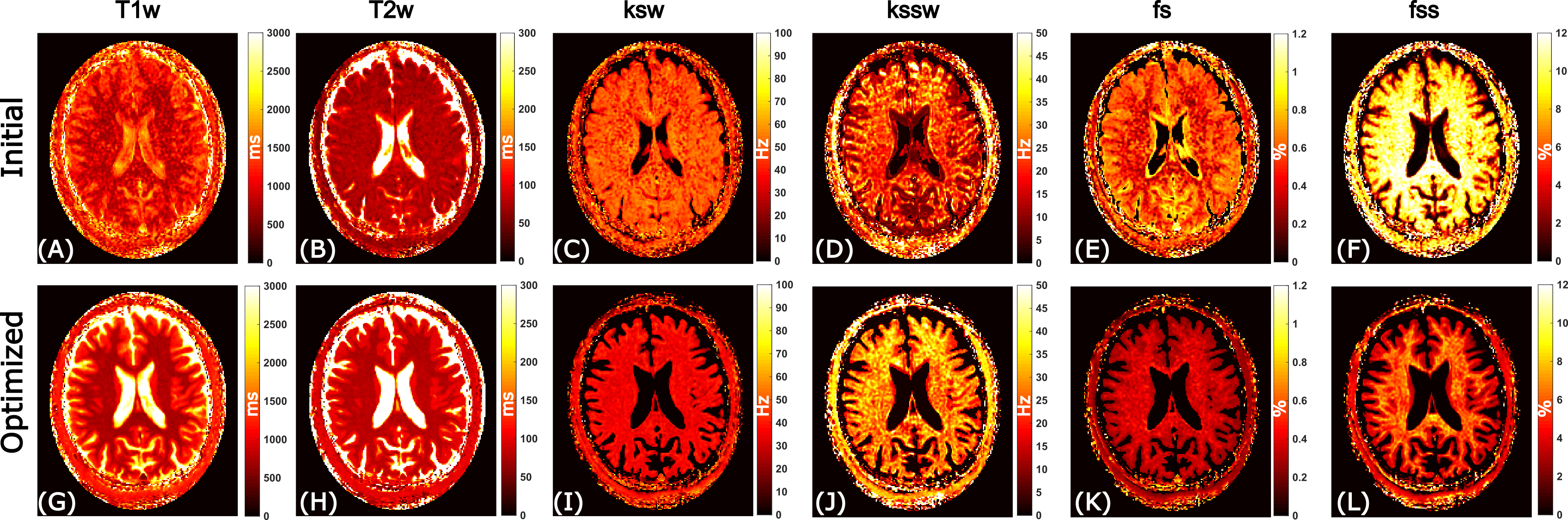
The initial and optimized schedules are shown in Figure 3. The optimized schedule resulted in a scan time that was 12% shorter than the initial random schedule (92 vs 105 seconds). The effect of SNR on the two schedules tested in the phantom is shown in Figure 4, where the optimized schedule provided a similar or lower error. In vivo CEST-MRF quantitative maps in the healthy subject are presented in Figure 5. Despite the 12% shorter acquisition time, the sequence with the optimized schedule presented tissue maps with improved image quality and good agreement to literature values [2].Discussion
Previous MRF optimization methods used proxy measures of optimality rather than actual reconstruction error and were limited to a small number of acquisition and/or tissue parameters [11]–[13]. More recent DL approaches rely on back-propagation of the loss to update both the acquisition parameters and the network weights in each epoch [14]–[16]. However, since network learning is nonlinear, the loss in each epoch may not reflect the true reconstruction error (Figure 1D) and lead to sub-optimal schedules. To address this weakness, the DL approach presented in this work calculated the reconstruction error only after the network was trained to convergence. The acquisition schedule optimization proposed in this work is widely applicable and can be used to optimize MRF sequences in general.Conclusion
This work demonstrated a DL approach to optimize the acquisition schedule of CEST-MRF in the human brain with 12% scan acceleration and improved image quality compared to a conventional acquisition schedule. Future work will test the application to brain tumors, including reproducibility analysis.Acknowledgements
This work was supported by NIH/NCI grants P30-CA008748 and R37CA262662-01A1.References
[1] O. Cohen, S. Huang, M. T. McMahon, M. S. Rosen, and C. T. Farrar, “Rapid and quantitative chemical exchange saturation transfer (CEST) imaging with magnetic resonance fingerprinting (MRF),” Magnetic resonance in medicine, vol. 80, no. 6, pp. 2449–2463, 2018.
[2] O. Cohen et al., “CEST MR Fingerprinting (CEST-MRF) for Brain Tumor Quantification Using EPI Readout and Deep Learning Reconstruction,” Magnetic Resonance in Medicine, 2022.
[3] O. Cohen, “MR Fingerprinting Schedule Optimization Network (MRF-SCONE),” in Proceedings of the International Society of Magnetic Resonance in Medicine, Montreal, May 11-May 16, p. 4531.
[4] O. Perlman, C. T. Farrar, and O. Cohen, “Deep Learning Global Schedule Optimization for Chemical Exchange Saturation Transfer MR Fingerprinting (CEST-MRF),” in Proceedings of the International Society of Magnetic Resonance in Medicine, Virtual Conference, Aug. 2020, p. 3576.
[5] J.-S. Park, “Optimal Latin-hypercube designs for computer experiments,” Journal of statistical planning and inference, vol. 39, no. 1, pp. 95–111, 1994.
[6] O. Cohen, B. Zhu, and M. S. Rosen, “MR fingerprinting deep reconstruction network (DRONE),” Magnetic resonance in medicine, vol. 80, no. 3, pp. 885–894, 2018.
[7] D. P. Kingma and J. Ba, “Adam: A method for stochastic optimization,” arXiv preprint arXiv:1412.6980, 2014.
[8] A. Mayer, T. Mora, O. Rivoire, and A. M. Walczak, “Diversity of immune strategies explained by adaptation to pathogen statistics,” Proceedings of the National Academy of Sciences, vol. 113, no. 31, pp. 8630–8635, 2016.
[9] J. C. Spall, “Implementation of the simultaneous perturbation algorithm for stochastic optimization,” IEEE Transactions on aerospace and electronic systems, vol. 34, no. 3, pp. 817–823, 1998.
[10] D. L. Collins et al., “Design and construction of a realistic digital brain phantom,” IEEE transactions on medical imaging, vol. 17, no. 3, pp. 463–468, 1998.
[11] O. Cohen and M. S. Rosen, “Algorithm comparison for schedule optimization in MR fingerprinting,” Magnetic resonance imaging, vol. 41, pp. 15–21, 2017.
[12] B. Zhao et al., “Optimal experiment design for magnetic resonance fingerprinting: Cramer-Rao bound meets spin dynamics,” IEEE transactions on medical imaging, vol. 38, no. 3, pp. 844–861, 2018.
[13] O. Perlman, K. Herz, M. Zaiss, O. Cohen, M. S. Rosen, and C. T. Farrar, “CEST MR-Fingerprinting: practical considerations and insights for acquisition schedule design and improved reconstruction,” Magnetic resonance in medicine, vol. 83, no. 2, pp. 462–478, 2020.
[14] B. Kang, B. Kim, H. Park, and H.-Y. Heo, “Learning-based optimization of acquisition schedule for magnetization transfer contrast MR fingerprinting,” NMR in Biomedicine, vol. 35, no. 5, p. e4662, 2022.
[15] O. Perlman, B. Zhu, M. Zaiss, M. S. Rosen, and C. T. Farrar, “An end-to-end AI-based framework for automated discovery of rapid CEST/MT MRI acquisition protocols and molecular parameter quantification (AutoCEST),” Magnetic Resonance in Medicine, vol. 87, no. 6, pp. 2792–2810, 2022.
[16] P. K. Lee, L. E. Watkins, T. I. Anderson, G. Buonincontri, and B. A. Hargreaves, “Flexible and efficient optimization of quantitative sequences using automatic differentiation of Bloch simulations,” Magnetic resonance in medicine, vol. 82, no. 4, pp. 1438–1451, 2019.
Figures