2181
A steady-state MRF sequence optimization framework for 3D simultaneous water T1 and fat fraction mapping1NMR Laboratory, Neuromuscular Investigation Center, Institute of Myology, Paris, France
Synopsis
Keywords: MR Fingerprinting/Synthetic MR, MR Fingerprinting
We introduce an optimization framework using the longitudinal steady-state equilibrium for FLASH MRF sequences, and taking into account signal noise by using a Monte Carlo method. We use this framework to optimize echo times, flip angles, timings and recovery time for T1H2O and FF mapping while shortening our original MRF T1-FF sequence. The resulting Fast MRF T1-FF sequence yields comparable estimation results to the original sequence with an almost twice reduced acquisition time.Introduction
In the field of neuromuscular disorders (NMD), fat fraction (FF) is an established biomarker of disease severity and water T1 (T1H2O) has been shown to be a potential biomarker of disease activity [1]. The use of MR Fingerprinting (MRF) enables the simultaneous quantification of various parameters, such as FF and T1H2O [2]. However FLASH T1 MRF sequences (such as MRF T1-FF proposed in [3]) generally require long recovery times between repetitions for allowing the longitudinal magnetization to grow back to equilibrium. Shortening the sequence would highly benefit 3D imaging, where multiple acquisitions of the MRF scheme are required to encode along the partition encoding direction. However a shorter sequence is likely to degrade the parameter estimation quality. Hence we need to optimize the acquisition parameters of our shortened sequence for maintaining the quality of FF and T1H2O quantification.In this work, we introduced an optimization framework that takes into account the longitudinal steady-state equilibrium of the MRF sequence and handles acquisition noise using Monte Carlo simulations [4]. Through this framework, we optimized the echo times (TE), flip angles (FA) and recovery time of the MRF T1-FF sequence and compared the mapping accuracy and precision to the original implementation.
Methods
The optimization framework consisted of 4 blocks : i) a simulation block for steady-state MRF FLASH sequences with intial inversion pulse and variable TE,TR and FA, ii) an MRF pattern matching algorithm, iii) a cost function taking into account noise and iv) an optimizer (see Fig [1]).Regarding the MRF FLASH simulation block, for N impulsions with flip angles (θi)i=1..N of phase (φi)i=1..N, echo times (TEi)i=1..N and repetitions times (TRi)i=1..N, the magnetization has the following dynamics:
$$
M_x(t+TE_i)=M_z(t)sin(\theta_i)sin(\phi_i)e^{⁻\frac{TE_i}{T_2}}\\M_y(t+TE_i)=-M_z(t)sin(\theta_i)cos(\phi_i)e^{⁻\frac{TE_i}{T_2}}\\M_z(t+TR_i)=M_0+(M_z(t)cos(\theta_i)-M_0)e^{⁻\frac{TR_i}{T_1}}
$$
$$$m_p=M_z(p*T)$$$ represents the initial magnetization after p repetitions of the MRF scheme, where T is the total duration of the sequence.
We have :
$$m_p=Am_{p-1}+B$$
with $$$A=\prod_{i=1}^N{e^{⁻\frac{TR_i}{T_1}}cos(\theta_i)}$$$ and $$$B=M_0\sum_{i=0}^{N-1}{(1-e^{⁻\frac{TR_{N-i}}{T_1}})\prod_{j=N-i}^N{e^{⁻\frac{TR_j}{T_1}}cos(\theta_j)}}$$$.
$$$m_p$$$ is an arithmetic-geometric sequence with A<<1. Hence it reaches a steady-state after very few repetitions of the sequence, and the steady-state value is equal to B/(1-A).
MRF is mainly impacted by noise due to undersampling that we approximated with a Gaussian distribution representing an average SNR of 20. For pattern matching, we used exhaustive search into a bicomponent dictionary of fingerprints [5].
The following cost function was calculated to assess parameters mapping accuracy ([4]) :
$$C((\theta_i)_{i=1..N},(TE_i)_{i=1..N},TR_N)=\lambda_{T1}\frac{1}{N_s}\sum_{s=1}^{N_s}{\frac{|\widehat{T1_{H_2O}^s}-T1_{H_2O}^s|}{T1_{H_2O}^s}}+\lambda_{FF}\frac{1}{N_s}\sum_{s=1}^{N_s}|\widehat{FF^s}-FF^s|+\lambda_{T}\sum_{i=1}^{N}{TR_i}$$
where $$$T1_{H_2O}^s,FF^s $$$(resp.$$$\widehat{T1_{H_2O}^s},\widehat{FF^s}$$$ ) are the ground truth (resp. estimated) parameters for each simulated signal and Ns is the total number of simulated signals. We fixed N=760 spokes, the smallest number of spokes for which estimation did not worsen drastically. As using 760 spokes instead of 1400 spokes already reduced the sequence duration, we used $$$ \lambda_{T}=0$$$. $$$\lambda_{T1}$$$ and $$$\lambda_{FF}$$$ were set empirically to 1 and 2 for those terms to have similar order of magnitudes.
To reduce the dimension of the problem, we assumed that TE and FA had piecewise constant evolutions with respectively 3 and 5 pieces, and that (TRi)i=1..(N-1) were kept at their minimum possible value allowed by the gradient system and bandwidth, which left us with a total of 15 parameters to optimize for : Flip angles values (θi)i=1..N , echo time values (TEi)i=1..N, breaks timings and recovery time TRN at the end of each repetition.
The signals were simulated for the following grid of tissue parameters : T1H2O =500:100:1900 (ms), FF = 0.:0.1:0.5, df = [-30.,0,30] (Hz), B1=[0.7,1.0].
The algorithm used for minimizing the cost function was differential evolution [6], which is an efficient global optimization method when the gradient of the cost function is not easily accessible. The maximum functions evaluations was set at 150000 but the algorithm stopped earlier.
We compared the reference (MRF T1-FF) and optimal (Fast MRF T1-FF) sequences on 3D numerical phantoms (16 slices – 64 square subregions of size 4x4 per slice with randomly varying T1H2O, FF, Df and B1) and 3D in vivo data acquired at 3T (PrismaFit, Siemens Healthineers) on the thighs of one healthy control (20 partitions, resolution 1x1x5 mm3, FOV 10x40x40cm3,10 regions of interest (ROIs) drawn on the left thigh muscles).
Results
Each repetition of Fast MRF T1-FF lasts 6.5s against 10.9s for MRF T1-FF (Fig [2]). The recovery of 3s at the end of each repetition did not allow for the longitudinal magnetization to grow back to intial equilibrium, however the steady-state was reached after a maximum of two repetitions of the Fast MRF T1-FF sequence (Fig [3]).On numerical phantoms, T1H2O and FF estimation accuracy and precision were similar to the reference sequence (Figure 4).
On in vivo data, accuracy was comparable to MRF T1-FF. Precision was degraded for T1H2O, with a 40 ms increase in standard deviation on average (Figure 5).
Discussion & Conclusion
Using a new optimization framework taking into account steady-state magnetization and noise, we designed a new sequence (Fast T1-FF MRF) for fast quantification of T1H2O and FF, with reduced time and comparable results to those of the reference sequence. In vivo, the new sequence was less precise, however this could be alleviated by MRF denoising techniques ([7]).The explicit calculation of the steady-state value removed the need to simulate several repetitions of the MRF sequence and allowed to reduce the computation time for sequence optimization.
Acknowledgements
This study was funded by ANR-20-CE19-0004.References
[1] Marty, B., Reyngoudt, H., Boisserie, J. M., le Louër, J., Araujo, E. C. A., Fromes, Y., & Carlier, P. G. (2021). Water-fat separation in mr fingerprinting for quantitative monitoring of the skeletal muscle in neuromuscular disorders. Radiology, 300(3), 652–660. https://doi.org/10.1148/radiol.2021204028
[2] Ma, D., Gulani, V., Seiberlich, N., Liu, K., Sunshine, J. L., Duerk, J. L., & Griswold, M. A. (2013). Magnetic resonance fingerprinting. Nature, 495(7440), 187–192. https://doi.org/10.1038/nature11971
[3] Marty, B., Lopez Kolkovsky, A. L., Araujo, E. C. A., & Reyngoudt, H. (2021). Quantitative Skeletal Muscle Imaging Using 3D MR Fingerprinting With Water and Fat Separation. Journal of Magnetic Resonance Imaging, 53(5), 1529–1538. https://doi.org/10.1002/jmri.27381
[4] Karsten S. et al. (2016). Towards judging the encoding capability of Magnetic Resonance Fingerprinting sequences. ISMRM Proc 2016
[5] Slioussarenko, C., Baudin ,P.Y. , Reyngoudt, H. & Marty, B (2022). Bi-component dictionary for efficient quantification of fat fraction and water T1 via MR fingerprinting. ISMRM Proc 2022
[6] Storn, R., & Price, K. (1997). Differential Evolution-A Simple and Efficient Heuristic for Global Optimization over Continuous Spaces. Journal of Global Optimization, 11, 341–359.
[7] Mazor, G., Weizman, L., Tal, A., & Eldar, Y. C. (2018). Low-rank magnetic resonance fingerprinting. https://doi.org/10.1002/mp.13078 p { margin-bottom: 0.25cm; direction: ltr; line-height: 115%; text-align: left; orphans: 2; widows: 2; background: transparent }a:link { color: #0563c1; text-decoration: underline }
Figures
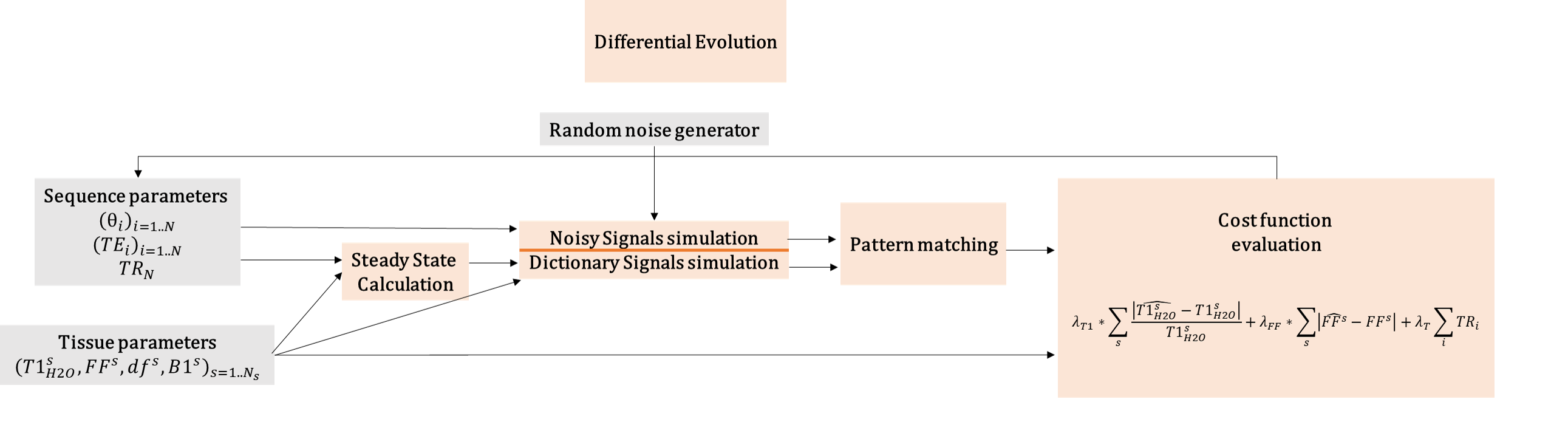
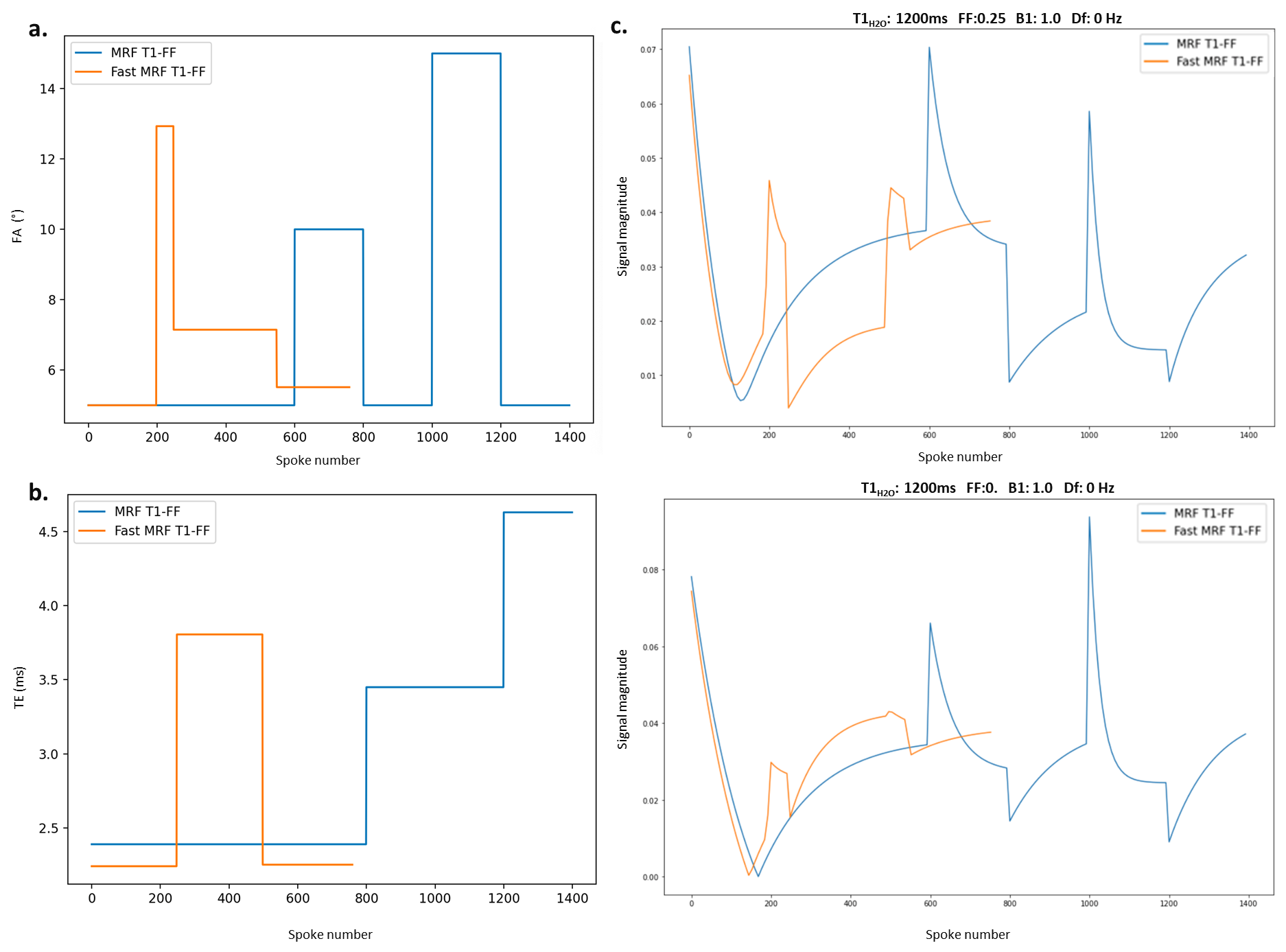
Fig.2:
a. Flip angle (FA) evolution for MRF T1-FF and Fast MRF T1-FF
b. Echo time (TE) evolution for MRF T1-FF and Fast MRF T1-FF
c. Magnitude of example fingerprints for MRF T1-FF and Fast MRF T1-FF for 2 sets of parameters
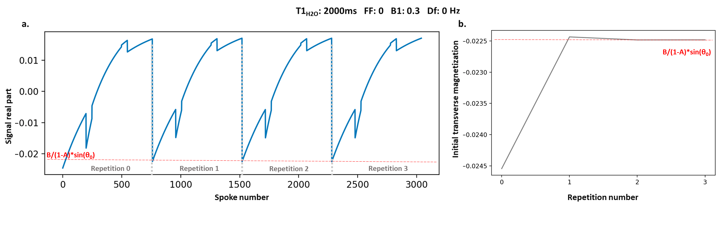
Fig.3 : Fingerprint with highest T1H2O and lowest B1 - hence taking the most time to reach longitudinal steady-state.
a. Real part of the fingerprint as a function of spoke number for first 4 repetitions, with the calculated steady-state value in red
b. Initial transversal magnetization as a function of repetition, with the calculated steady-state value in red. The steady-state was reached after 2 repetitions.
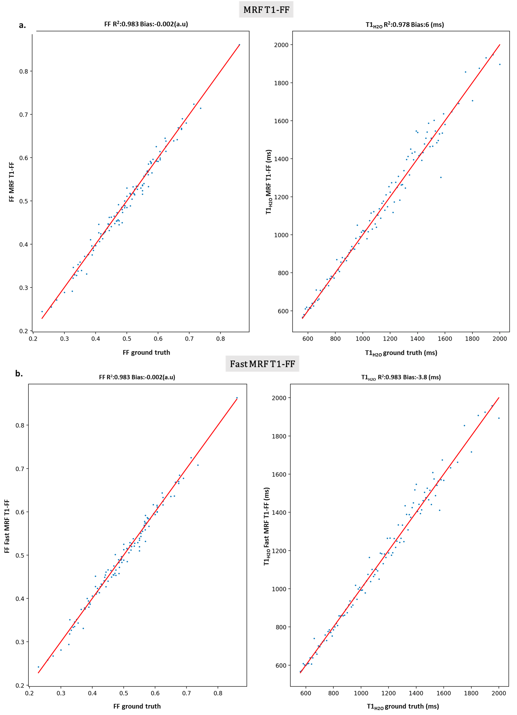
Fig.4 : FF and T1H2O parameter estimation accuracy and precision for MRF T1-FF and Fast MRF T1-FF on the ROIs of our square numerical phantom (regions with constant T1H2O values).
The accuracy and precision were very similar between both sequences, and the accuracy was even a bit better for T1H2O with the new sequence.
a. MRF T1-FF regression plot of FF and T1H2O on all ROIs against ground truth
b. Fast MRF T1-FF regression plot of FF and T1H2O on all ROIs against ground truth
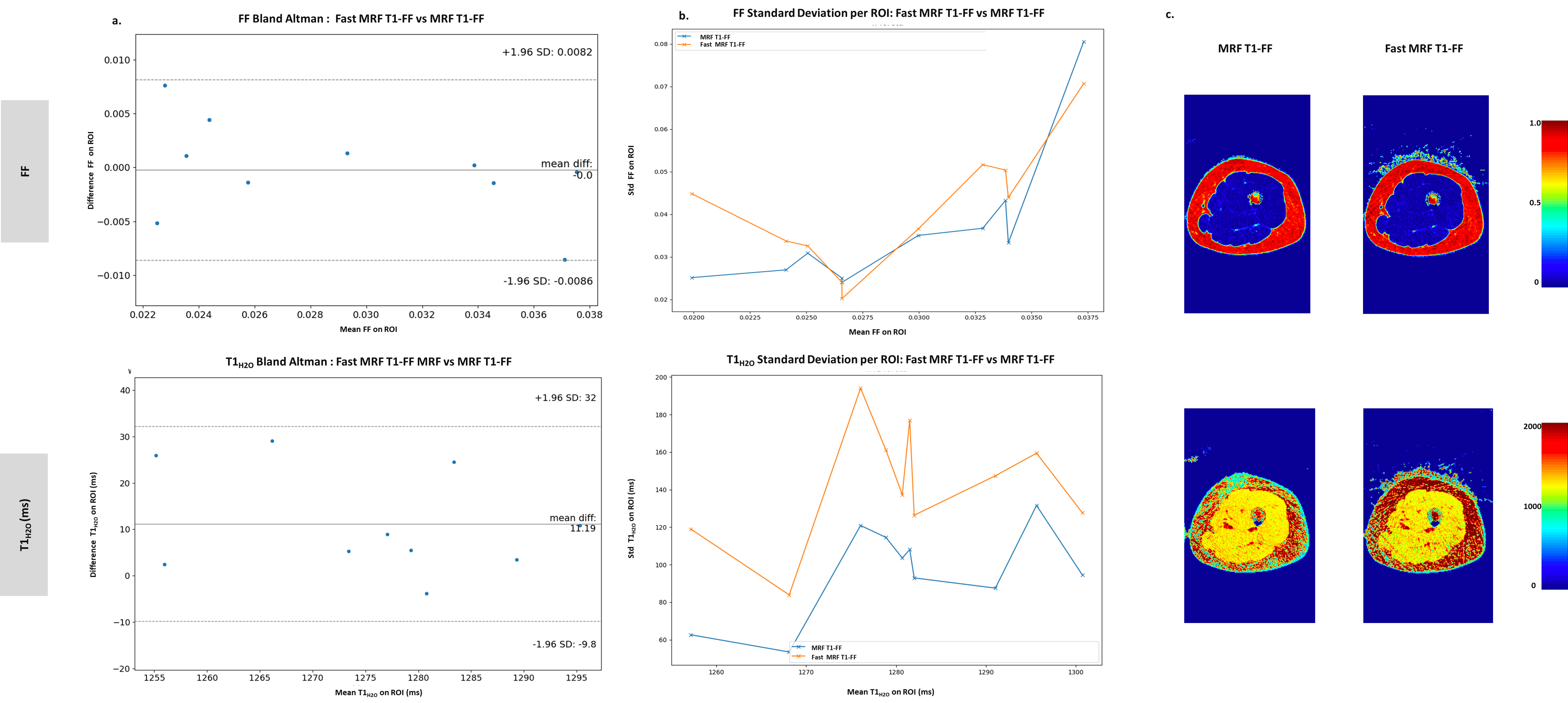
Fig.5 : In vivo comparison of Fast MRF T1-FF and MRF T1-FF on the 10 ROIs drawn in the left thigh muscles of one healthy control.
a. Bland Altman plots for T1H2O and FF in each ROIs of Fast MRF T1-FF against MRF T1-FF. The new sequence yielded comparable results in term of accuracy as the reference sequence, with no visible bias.
b. Standard deviation (std) of T1H2O and FF estimation in each ROIs of both sequences. FF precision was similar for both sequences, whereas T1H2O precision was slightly degraded (40ms average std increase).
c. Example FF and T1H2O maps for both sequences on one axial slice