2175
A New Framework for 3D MR Fingerprinting with Efficient Subspace Reconstruction and Joint Posterior Distribution Estimation1Department of Radiation Oncology, University of Michigan, Ann Arbor, MI, United States, 2Department of Biomedical Engineering, University of Michigan, Ann Arbor, MI, United States, 3Department of Radiology, University of Michigan, Ann Arbor, MI, United States
Synopsis
Keywords: MR Fingerprinting/Synthetic MR, MR Fingerprinting
Iterative image reconstruction of highly undersampled high-resolution 3D MR fingerprinting (MRF) is time-consuming and has high memory requirements. In this work, we propose to use stochastic gradient descent to accelerate the reconstruction and reduce the memory footprint. In addition, a conditional invertible neural network is used as a fast and flexible tool for estimating the posterior distribution of tissue properties from MRF. In a simulation study, we achieved an 11-fold and 45.5GB reduction in reconstruction time and memory requirement, respectively, compared with a conventional iterative method. Uncertainty maps of tissue properties derived from the estimated posterior distributions correlate well with reconstruction errors.
Introduction
3D MR fingerprinting (MRF)1 has been proposed for 3D tissue property mapping. However, highly accelerated 3D high-resolution MRF requires iterative reconstruction from large-scale MR data which comes with a high computation expense and long reconstruction times, thus limiting its clinical translation. In addition, a fast and flexible approach to estimate posterior distribution of tissue properties, which may provide uncertainty measures for downstream tasks, such as lesion detection2, has not been developed for MRF. In this work, we propose a framework to efficiently reconstruct parameter maps and posterior distributions for 3D high-resolution MRF.Methods
Our 3D MRF reconstruction framework (Figure 1) consists of two major components:1) TR-decomposed stochastic gradient decent (SGD) subspace reconstruction to build coefficient maps of principle components of MRF-time series and 2) a conditional invertible neural network (cINN)3 to estimate parameter maps and their posterior distributions.MRF subspace reconstruction has been proposed to reconstruct spatial coefficient maps of k temporal basis functions obtained by principal component analysis (PCA) of a dictionary of MRF signals with T TRs (k<<T)4. The reconstruction can be posed as an optimization problem as follows:$$\hat{c}=argmin_c||F_{NU}Sc\Phi-y||_2^2+\lambda(c),$$ where $$$c\in\mathbb{C}^{N\times k}$$$ denotes spatial bases, $$$\Phi\in\mathbb{C}^{k\times T}$$$ denotes temporal bases from PCA, $$$S\in\mathbb{C}^{N_cN\times N}$$$ denotes coil sensitivity maps, $$$F_{NU}\in\mathbb{C}^{(N_cM\times T)\times(N_cN\times T)}$$$ is the non-uniform FFT(NUFFT) operator, $$$y\in\mathbb{C}^{N_cM\times T}$$$ represents acquired k-space data, $$$\lambda R(\cdot)$$$ is a regularization on spatial bases. $$$N$$$ is the spatial size of image, $$$N_c$$$ is the number of coils and $$$M$$$ is the number of k-space acquisitions per TR. Conventionally, iterative reconstructions require the gradient of the data consistency term $$$S'F_{NU}'(F_{NU}Sc\Phi-y)\Phi'$$$, to be calculated at each iteration. This involves applying a 3D NUFFT operation for each TR and coil, which results in a prohibitively slow optimization. To circumvent these issues, in this work, we propose to use SGD to accelerate the reconstruction5 and decompose the optimization objective in the TR dimension as a sum over T TRs:$$\hat{c}=argmin_c\sum^T_{t=1}L_t(c)=argmin_c\sum^T_{t=1}||F^t_{NU}Sc\Phi_t-y_t||_2^2+\frac{\lambda}{T}R(c),$$where $$$F_{NU}^t$$$, $$$\Phi_t$$$, and $$$y_t$$$ are the NUFFT operator, temporal bases, and k-space data at the tth TR, respectively. At each iteration, one TR is selected, and c is updated as $$$c=c-\alpha T\nabla_cL_t(c)$$$, where $$$\alpha$$$ is the step size. This modification greatly reduces the memory requirements and computation time for each iteration.
The cINN3 that was originally proposed to solve highly degenerate inverse problems in astrophysics6,7 is used here to estimate parameter maps and their posterior distributions. Given pairs of tissue parameters and corresponding noisy MR signals, the network learns to minimize the Kullback-Leibler divergence between the estimated and true posterior distributions. The cINN is flexible in the sense that it can be readily trained and adapted for different reconstruction methods with different noise statistics.
To validate the proposed image reconstruction method, 20 digital brain phantoms8 were reformatted to 1mm-isotropic resolution with a field of view of 230×230×230mm3. The MRF signals were simulated voxel-by-voxel with a truncated FISP-based MRF sequence9 (500TRs). Coil sensitivity maps with 8 coils and complex Gaussian noise (SNR=30) were simulated. The images were retrospectively undersampled in k-space using a 3D multi-axis spiral projection trajectory10 with 8 acquisition groups (total scan time=61s). Total variation regularization was used with $$$\lambda=1\times 10^{-9}$$$. Five principal components were retained.
The cINN was trained on a dictionary of MRF signals simulated using T1=[20:10:4000]ms and T2=[2:2:1200]ms with added Gaussian noise, called here "vanilla cINN". 50%/30%/20% of the data were randomly selected for training/validation/testing. We validated the estimated posterior distribution by comparing it with a Markov chain Monte Carlo (MCMC) method11 using 20000 samples. The normalized root mean squared errors (NRMSEs) of the estimates were compared to two neural network-based point estimation methods, FCNN12 and RNN13. Another cINN was trained on the SGD reconstruction of 8 digital phantoms, dubbed adaptive cINN, to adapt to the noise statistics of the reconstruction and the prior distribution of tissue properties in brain.
Finally, the SGD subspace reconstruction was combined with either the vanilla or adaptive cINN, which were compared to 1) adjoint NUFFT image reconstruction followed by pattern matching and 2) locally low rank (LLR) regularized iterative subspace reconstruction10 followed by the vanilla cINN.
Results
The vanilla cINN estimated posterior distributions which were similar to ones estimated via MCMC (Figure 2), but with much faster computation speed (0.81 seconds per voxel vs ~60 minutes for MCMC). The vanilla cINN, while providing posterior distributions, achieved NRMSEs of T1 and T2 comparable to FCNN, but better than RNN (Table 1). Figure 3 shows comparisons of the parameter maps of one example slice using different reconstruction methods. The SGD+vanilla cINN shows better visual quality than pattern matching and LLR+vanilla cINN. Compared with LLR, SGD reconstruction achieved respective 11-fold and 45.5GB reductions in computation time (25min vs. 4.4hours) and memory (9.5GB vs. 55GB). The adaptive cINN further improved parameter estimation, and the uncertainty maps visually correlate with the estimation error.Discussion and conclusion
Our method was able to efficiently estimate the posterior distribution and perform subspace reconstruction for 3D MRF, while maintaining accurate recovery of tissue property maps and significantly reducing memory requirements and reconstruction time. Unrolling the SGD algorithm paves the path towards deep learning-based reconstruction. Also, the cINN can characterize encoding capabilities of a MRF sequence and may aid in sequence design.Acknowledgements
This work was supported by NIH R01 EB016079.References
1. Ma D, Jiang Y, Chen Y, et al. Fast 3D magnetic resonance fingerprinting for a whole-brain coverage. Magn Reson Med. 2018;79(4):2190-2197. doi:10.1002/mrm.26886
2. Ma D, Jones SE, Deshmane A, et al. Development of high-resolution 3D MR fingerprinting for detection and characterization of epileptic lesions. Journal of Magnetic Resonance Imaging. 2019;49(5):1333-1346. doi:10.1002/jmri.26319
3. Ardizzone L, Kruse J, Lüth C, Bracher N, Rother C, Köthe U. Conditional Invertible Neural Networks for Diverse Image-to-Image Translation. Published online May 5, 2021. http://arxiv.org/abs/2105.02104
4. Zhao B, Setsompop K, Adalsteinsson E, et al. Improved magnetic resonance fingerprinting reconstruction with low-rank and subspace modeling. Magn Reson Med. 2018;79(2):933-942. doi:10.1002/mrm.26701
5. Ong F, Zhu X, Cheng JY, et al. Extreme MRI: Large-scale volumetric dynamic imaging from continuous non-gated acquisitions. Magn Reson Med. 2020;84(4):1763-1780. doi:10.1002/mrm.28235
6. Kang DE, Pellegrini EW, Ardizzone L, et al. Emission-line diagnostics of HII regions using conditional Invertible Neural Networks. Published online January 21, 2022. doi:10.1093/mnras/stac222
7. Haldemann J, Ksoll V, Walter D, et al. Exoplanet Characterization using Conditional Invertible Neural Networks. Published online January 31, 2022. http://arxiv.org/abs/2202.00027
8. Aubert-Broche B, Griffin M, Pike GB, Evans AC, Collins DL. Twenty new digital brain phantoms for creation of validation image data bases. IEEE Trans Med Imaging. 2006;25(11):1410-1416. doi:10.1109/TMI.2006.883453
9. Jiang Y, Ma D, Seiberlich N, Gulani V, Griswold MA. MR fingerprinting using fast imaging with steady state precession (FISP) with spiral readout. Magn Reson Med. 2015;74(6):1621-1631. doi:10.1002/mrm.25559
10. Cao X, Liao C, Iyer SS, et al. Optimized multi‐axis spiral projection <scp>MR</scp> fingerprinting with subspace reconstruction for rapid whole‐brain high‐isotropic‐resolution quantitative imaging. Magn Reson Med. Published online February 24, 2022. doi:10.1002/mrm.29194
11. Haario H, Saksman E, Tamminen J. An Adaptive Metropolis Algorithm. Bernoulli. 2001;7(2):223. doi:10.2307/3318737
12. Cohen O, Zhu B, Rosen MS. MR fingerprinting Deep RecOnstruction NEtwork (DRONE). Magn Reson Med. 2018;80(3):885-894. doi:10.1002/mrm.27198
13. Oksuz I, Cruz G, Clough J, et al. Magnetic Resonance Fingerprinting Using Recurrent Neural Networks. In: 2019 IEEE 16th International Symposium on Biomedical Imaging (ISBI 2019). IEEE; 2019:1537-1540. doi:10.1109/ISBI.2019.8759502
Figures
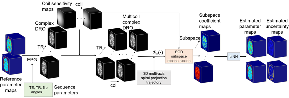
Figure 1. The overall pipeline of the proposed method. 1mm-isotropic resolution digital reference objects (DROs) for brain were created and used for experiment. Our 3D MRF reconstruction framework consists of two major components: 1) TR-decomposed stochastic gradient decent (SGD) subspace reconstruction, which is fast and memory efficient, and 2) a conditional invertible neural network (cINN) to accurately estimate both parameter maps and corresponding posterior distributions.
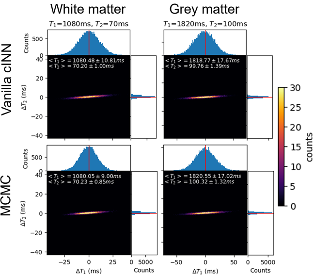
Figure 2. The estimated posterior distributions of T1 and T2 from two noisy MRF signal-time courses simulated using typical white (first column) and grey (second column) matter T1 and T2 values using vanilla cINN (first row) and MCMC (second row). The x- and y- axes of each panel show the deviation from the ground truth T1 and T2 values. The projections onto x- and y- axes represent the marginal distribution of T1 and T2, respectively. The empirical means and standard deviations of T1 and T2 are shown in the top left corner of each plot.
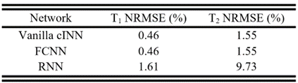
Table 1. NRMSE (%) of T1 and T2 estimated by vanilla cINN, FCNN, and RNN on the testing set. While cINN can provide posterior distribution of tissue properties, it performed on par with FCNN and better than RNN.
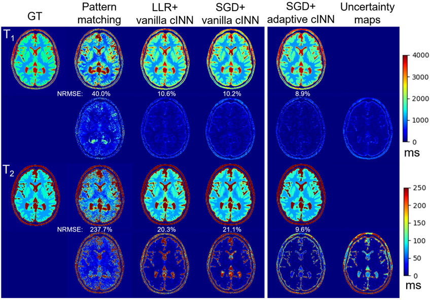
Figure 3. Ground truth (GT) (first column) T1 (first row) and T2 (third row) maps and reconstructions from one example slice using pattern matching (second column), LLR reconstruction (third column), SGD reconstruction followed by vanilla cINN (fourth column) and adaptive cINN (fifth column). The difference maps compared to the GT are shown in the second and fourth row for T1 and T2, respectively, with NRMSE values shown on the top. The uncertainty maps calculated by standard deviations of the posterior distributions of T1 and T2 for the SGD+adaptive cINN are shown in the last column.