2172
Whole Brain Spherical Mean Value Filtering for Shadow Reduction in Quantitative Susceptibility Mapping
Alexandra Grace Roberts1,2, Pascal Spincemaille2, Thanh Nguyen2, and Yi Wang1,2
1Electrical Engineering, Cornell University, Ithaca, NY, United States, 2Radiology, Weill Cornell Medicine, New York, NY, United States
1Electrical Engineering, Cornell University, Ithaca, NY, United States, 2Radiology, Weill Cornell Medicine, New York, NY, United States
Synopsis
Keywords: Quantitative Imaging, Artifacts
Morphology Enabled Dipole Inversion (MEDI) is an iterative reconstruction algorithm for Quantitative Susceptibility Mapping (QSM) that is effective in suppressing streaking artifacts by exploiting the magnitude image as a morphological prior. However, contiguous areas of dipole incompatibility (such as noise) induce shadow artifacts whose spatial frequency components are not sufficiently regularized by the gradient-based regularization in MEDI. The harmonic quality allows the use of the maximum corollary of Green’s theorem to remove residual background field. This mSMV approach reduces shadows and preserves brain volume, comparing favorably to existing algorithms.Introduction
Quantitative susceptibility mapping (QSM) is a magnetic resonance imaging (MRI) method to calculate tissue susceptibility from local field of the measured field acquired from complex gradient echo (GRE) images. Bayesian approaches like Morphology Enabled Dipole Inversion (MEDI) [1] use anatomical knowledge such as tissue edge voxels determined from the magnitude image to penalize the streaking artifacts arising from dipole-incompatible sources. Low-frequency shadow artifacts persist from local field estimation errors in regions with low signal-to-noise ratio (SNR) near air-tissue interfaces. Large background field near these regions causes signal dephasing giving poor phase SNR, complicating separation of background and tissue field. The brain edge is eroded from kernel overlap or for boundary condition fidelity. Cortical and basal regions near air-tissue interface are important for studying iron accumulation in neurodegenerative diseases [9-11]. Efforts to reduce shadow artifacts introduce erosion during background field removal [12, 13] or addressing voxels with low SNR [14, 15]. Other variations avoid erosion but reduce region-of-interest (ROI) accuracy [16, 17]. The Spherical Mean Value (SMV) property of harmonic background fields suppresses these artifacts by applying an SMV filter to the dipole kernel (MEDI-SMV) and the local field from background field removal algorithms such as Projection onto Dipole Fields (PDF) [18]. This approach requires brain erosion as the SMV operation cannot be applied where the kernel extends beyond the ROI. Variations of (Variable, Regularized) Sophisticated Harmonic Artifact Reduction for Phase data or (V, RE) SHARP, [19-22] reduce artifacts while preserving more brain volume. Erosion also results from background field removal methods such as Laplacian Boundary Value (LBV) assuming zero local field at the boundary [23]. An algorithm using the maximum corollary of Green’s theorem removes shadows while preserving brain volume, referred to as maximum Spherical Mean Value (mSMV).Theory
SMV operatorThe brain ROI mask is partitioned (Figure 1). Since the background field $$$b_B(r)$$$ is an order of magnitude larger than local field $$$b(r)$$$ , the measured field $$$b^*$$$ at the maximum, is assumed to contain residual background field - local field is overestimated. An initial SMV filtering operation is performed, $$b_{SMV} (r)=b_L (r)-(S_{(r=5)} b_L)(r)\tag{1}$$ Where the SMV operator is $$(S_{(r=5)} b)(r)= F^{-1} {Fb(r)}\odot \kappa_{(r=5)}\tag{2}$$ $$$F$$$ denotes the Fourier transform and $$$\odot$$$ point-wise multiplication with $$$\kappa$$$, the Fourier transform of the spherical kernel with radius $$$r$$$. $$$M_e$$$ is the edge mask of outer $$$5mm$$$ of brain volume. Conventionally, this is eroded because overlap of the kernel with zero voxels outside $$$M$$$ yields an underestimated background field - the local field at the edge is erroneously high.
Residual background field mask
Voxels with large field values within are considered residual background field according to $$M_{b_0}(r) = \begin{cases} 1 & \text{if $|b_{SMV}(r))|>t$} \\ 0 & \text{else} \\ \end{cases} \tag{3}$$ A voxel contains residual background field if the magnitude after SMV filtering exceeds threshold $$$t$$$, a function of the maximum, $$t=\mathrm{min}\left(\frac{S_{r'=r}(b^*))}{2},P_{90} S_{(r'=r)} M_e (r)\odot b_L (r)\right)\tag{4}$$ $$$P_{90}$$$ indicates the 90th percentile value of voxels at the edge (where the filtering operation did not remove residual background field). A threshold function of the maximum and 90th percentile ensures adequate residual background field is included in $$$M_{b_0}(r)$$$. The maximum corollary of Green’s theorem [24] ensures residual background field is found at the brain edge $$$M_e(r)$$$ $$\mathrm{max}_{(r∈R)}b_B (r) \in \partial R\tag{5}$$ Kernel overlap causes underestimation of the residual background field at the edge of the brain and gives overestimated local field. The mask is partitioned $$$M(r)=M_e(r) \cup M_{\sim e} (r)$$$ - the residual background field mask is a subset of the edge mask, $$$M_{b_0}(r) \subset M_e(r)$$$, and contains shadow-inducing residual background field.
Vessel mask
The vessel mask limits field values while preserving high-frequency content. Vessels are preserved by binarizing the high-pass filtered local field magnitude $$$(S_{(r=1)}b)(r)$$$ above 1/4th its standard deviation and excluded from $$$M_{b_0}(r)$$$. The overestimated local field is truncated above $$$P_{97}(M_{\sim e}(r))$$$ - the susceptibility of vessels outside the interior mask are truncated at the 97th percentile of vessel susceptibilities inside interior mask $$$M_{\sim e}$$$ where residual background field is correctly removed.
mSMV operator
The SMV operation iterates until $$$\frac{\sum_i M_{b_0}(i)}{\sum_i M(i)}$$$ is below $$$\alpha=10^{-16}$$$ (Figure 2). $$(S_{(r=5)} b)(r)= F^{-1} \left(F{M_{b_0}(r)\odot b(r)}\right)\odot \kappa_{(r=0.5)}\tag{6}$$
Method
Ten patients were scanned at 3T (GE Healthcare) using a 3D multi-echo spoiled gradient echo sequence. Acquisition parameters were FOV of $$$24 cm$$$, partial FOV factor of $$$0.8$$$, acquisition matrix $$$384\times384\times64$$$, flip angle $$$\alpha=15^{\circ}$$$, slice thickness $$$2 mm$$$, repetition time $$$TR = 52 ms$$$, $$$11$$$ echoes, first echo at $$$TE=4.1 ms$$$, $$$\Delta TE = 4.4 ms$$$, parallel imaging factor $$$2$$$, and scan time $$$\sim8 min$$$. Local fields were obtained via PDF and subjected to mSMV, SMV, LBV, and VSHARP removing residual background field. QSMs were reconstructed using MEDI-L1 with regularization parameter $$$\lambda_1=1000$$$ and whole head CSF regularization $$$\lambda_{CSF}=1000$$$. Shadow scores (variance within cortical gray matter) [25] using the SMV mask were calculated.Results
Shadow reduction (Figure 3,4) between mSMV was comparable to VSHARP and SMV and significant above a 99% confidence level when compared to PDF and LBV. Multiple comparisons were addressed by Bonferroni correction.Discussion
For harmonic background fields, the maximum corollary of Green’s theorem helps identify and remove residual background field. This approach reduces shadows and preserves brain volume, comparing favorably to existing algorithms.Acknowledgements
No acknowledgement found.References
- L. De Rochefort et al., "Quantitative susceptibility map reconstruction from MR phase data using bayesian regularization: Validation and application to brain imaging," Magnetic Resonance in Medicine, vol. 63, no. 1, pp. 194-206, 2010, doi: 10.1002/mrm.22187.
- L. Li and J. S. Leigh, "Quantifying arbitrary magnetic susceptibility distributions with MR," Magnetic Resonance in Medicine, vol. 51, no. 5, pp. 1077-1082, 2004, doi: 10.1002/mrm.20054.
- J. P. Marques and R. Bowtell, "Application of a fourier-based method for rapid calculation of field inhomogeneity due to spatial variation of magnetic susceptibility," (in English), Concept Magn Reson B, vol. 25b, no. 1, pp. 65-78, Apr 2005, doi: 10.1002/cmr.b.20034.
- Y. Wang and T. Liu, "Quantitative susceptibility mapping (QSM): Decoding MRI data for a tissue magnetic biomarker," Magn Reson Med, vol. 73, no. 1, pp. 82-101, Jan 2015, doi: 10.1002/mrm.25358.
- S. Wharton, A. Schäfer, and R. Bowtell, "Susceptibility mapping in the human brain using threshold-based k-space division," Magnetic Resonance in Medicine, vol. 63, no. 5, pp. 1292-1304, 2010, doi: 10.1002/mrm.22334.
- J. K. Choi, H. S. Park, S. Wang, Y. Wang, and J. K. Seo, "Inverse Problem in Quantitative Susceptibility Mapping," SIAM Journal on Imaging Sciences, vol. 7, no. 3, pp. 1669-1689, 2014, doi: 10.1137/140957433.
- Z. L. Youngwook Kee, Liangdong Zhou, Alexey Dimov, Junghun Cho, Ludovic de Rochefort, Jin Keun Seo, and Yi Wang, "Quantitative Susceptibility Mapping (QSM) Algorithms: Mathematical Rationale and Computational Implementations," IEEE Transactions on Biomedical Engineering, vol. 64, no. 11, pp. 2531-2545, 2017, doi: 10.1109/tbme.2017.2749298.
- L. Zhou, J. K. Choi, Y. Kee, Y. Wang, and J. K. Seo, "Dipole Incompatibility Related Artifacts in Quantitative Susceptibility Mapping," arXiv: Medical Physics, 2017. [Online]. Available: https://arxiv.org/abs/1701.05457.
- Y. Wang et al., "Clinical quantitative susceptibility mapping (QSM): Biometal imaging and its emerging roles in patient care," J Magn Reson Imaging, vol. 46, no. 4, pp. 951-971, Oct 2017, doi: 10.1002/jmri.25693.
- M. Azuma et al., "Lateral Asymmetry and Spatial Difference of Iron Deposition in the Substantia Nigra of Patients with Parkinson Disease Measured with Quantitative Susceptibility Mapping," AJNR Am J Neuroradiol, vol. 37, no. 5, pp. 782-8, May 2016, doi: 10.3174/ajnr.A4645.
- A. D. Schweitzer et al., "Quantitative susceptibility mapping of the motor cortex in amyotrophic lateral sclerosis and primary lateral sclerosis," AJR Am J Roentgenol, vol. 204, no. 5, pp. 1086-92, May 2015, doi: 10.2214/AJR.14.13459.
- A. V. Dimov et al., "Global cerebrospinal fluid as a zero‐reference regularization for brain quantitative susceptibility mapping," Journal of Neuroimaging, vol. 32, no. 1, pp. 141-147, 2022, doi: 10.1111/jon.12923.
- Z. Liu, P. Spincemaille, Y. Yao, Y. Zhang, and Y. Wang, "MEDI+0: Morphology enabled dipole inversion with automatic uniform cerebrospinal fluid zero reference for quantitative susceptibility mapping," Magnetic Resonance in Medicine, vol. 79, no. 5, pp. 2795-2803, 2018, doi: 10.1002/mrm.26946.
- C. Langkammer et al., "Fast quantitative susceptibility mapping using 3D EPI and total generalized variation," NeuroImage, vol. 111, pp. 622-630, 2015, doi: 10.1016/j.neuroimage.2015.02.041.
- A. W. Stewart et al., "QSMxT: Robust masking and artifact reduction for quantitative susceptibility mapping," Magnetic Resonance in Medicine, vol. 87, no. 3, pp. 1289-1300, 2022, doi: 10.1002/mrm.29048.
- Alexandra Roberts, Thanh Nguyen, Yi Wang, "MEDI-d: Downsampled Morphological Priors for Shadow Reduction in Quantitative Susceptibility Mapping," in International Society for Magnetic Resonance in Medicine, 05/2021 2021, no. Signal Representation, 2021. [Online]. Available: https://cds.ismrm.org/protected/21MPresentations/abstracts/2599.html.
- Alexandra Roberts, Thanh Nguyen, Yi Wang, "MEDI-FM: Field Map Error Guided Regularization for Shadow Reduction in Quantitative Susceptibility Mapping," in International Society for Magnetic Resonance in Medicine, 05/2022 2022, no. Signal Representation, 2022.
- T. Liu et al., "A novel background field removal method for MRI using projection onto dipole fields (PDF)," NMR in Biomedicine, vol. 24, no. 9, pp. 1129-1136, 2011, doi: 10.1002/nbm.1670.
- W. Li, B. Wu, and C. Liu, "Quantitative susceptibility mapping of human brain reflects spatial variation in tissue composition," NeuroImage, vol. 55, no. 4, pp. 1645-1656, 2011, doi: 10.1016/j.neuroimage.2010.11.088.
- F. Schweser, A. Deistung, B. W. Lehr, and J. R. Reichenbach, "Quantitative imaging of intrinsic magnetic tissue properties using MRI signal phase: An approach to in vivo brain iron metabolism?," NeuroImage, vol. 54, no. 4, pp. 2789-2807, 2011, doi: 10.1016/j.neuroimage.2010.10.070.
- H. Sun and A. H. Wilman, "Background field removal using spherical mean value filtering and Tikhonov regularization," Magnetic Resonance in Medicine, vol. 71, no. 3, pp. 1151-1157, 2014, doi: 10.1002/mrm.24765.
- Y. Wen, D. Zhou, T. Liu, P. Spincemaille, and Y. Wang, "An iterative spherical mean value method for background field removal in MRI," Magnetic Resonance in Medicine, vol. 72, no. 4, pp. 1065-1071, 2014, doi: 10.1002/mrm.24998.
- D. Zhou, T. Liu, P. Spincemaille, and Y. Wang, "Background field removal by solving the Laplacian boundary value problem," NMR in Biomedicine, vol. 27, no. 3, pp. 312-319, 2014, doi: 10.1002/nbm.3064.
- K. K. Roy, "Green’s Theorem in Potential Theory," Springer Berlin Heidelberg, pp. 307-327.
- P. S. Balasubramanian, P.
Spincemaille, L. Guo, W. Huang, I. Kovanlikaya and Y. Wang. iScience 2020 Vol.
23 Issue 10 Pages 101553. DOI: 10.1016/j.isci.2020.101553
Figures
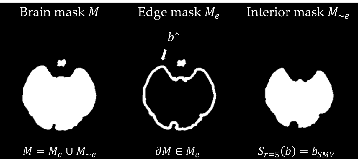
Figure 1. Mask partitioning into edge $$$M_e(r)$$$ and interior $$$M_{\sim e}(r)$$$. Local field is correctly calculated in $$$M_{\sim e}(r)$$$ and $$$M_e(r)$$$ is known to contain the maximum field value $$$b*$$$.
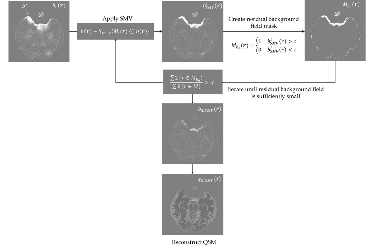
Figure 2. The mSMV algorithm.
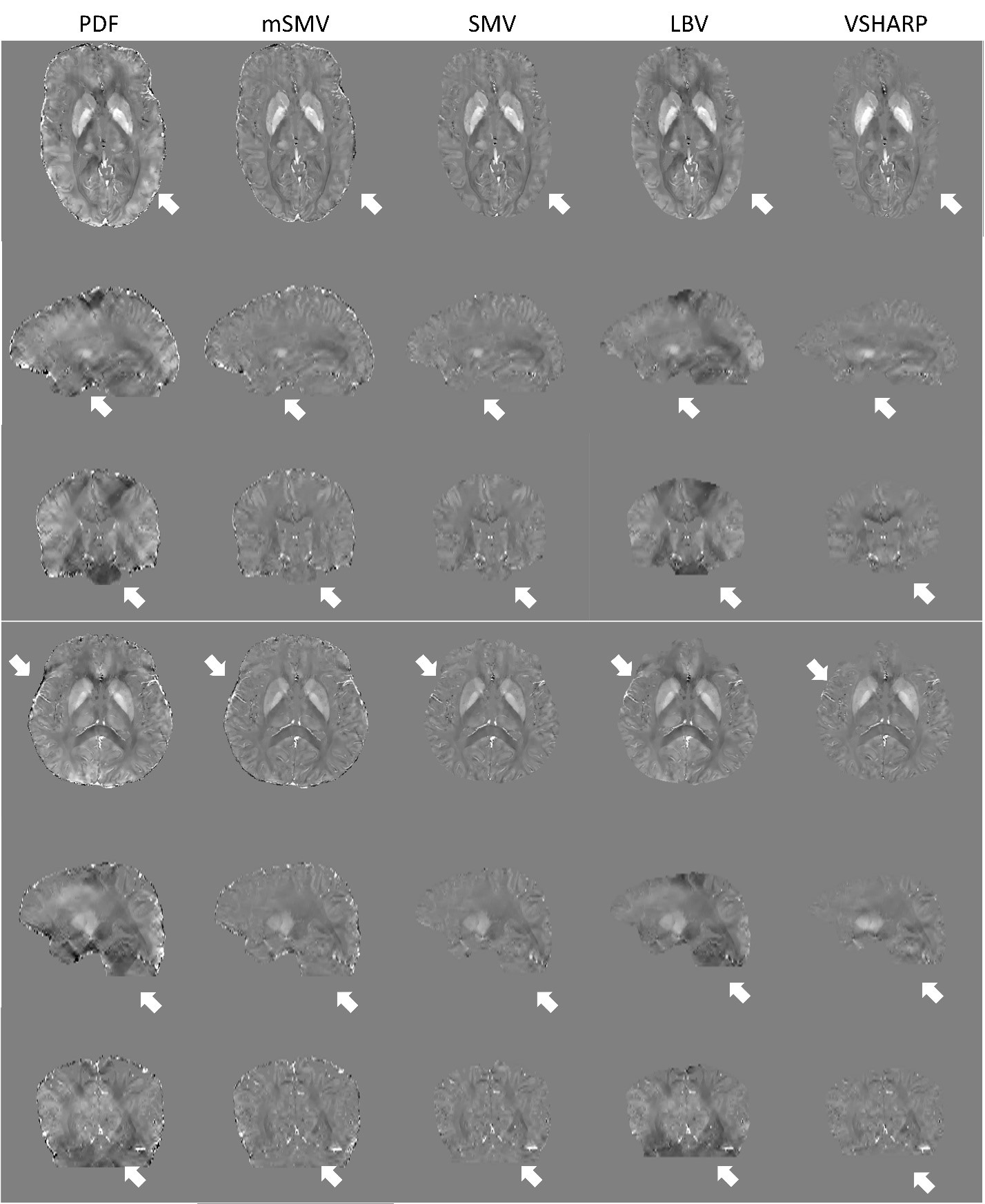
Figure
3. Healthy subjects QSMs, mSMV both reduces shadows and preserves the edge of
the brain.
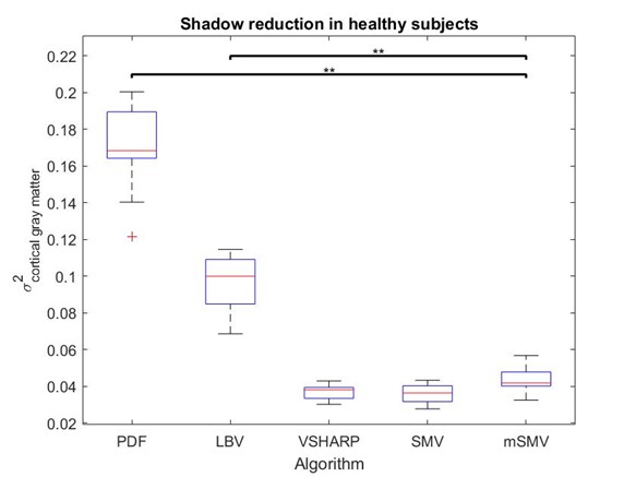
Figure 4. Cortical gray matter
variance within healthy subject reconstructions. Minimal shadow artifacts
correspond to minimal gray matter variance, as seen with mSMV.
DOI: https://doi.org/10.58530/2023/2172