2129
An investigation into the derangement of the linear relationship between 1/T1 and 1/H2O in brain tumours1Institute of Neuroradiology, University Hospital Frankfurt, Frankfurt, Germany, 2University Cancer Center Frankfurt (UCT), Frankfurt, Frankfurt, Germany, 3Frankfurt Cancer Institute (FCI), Frankfurt, Germany, 4German Cancer Research Center (DKFZ) and German Cancer Consortium (DKTK), Heidelberg, Germany, 55 Brain Imaging Center, Goethe University, Frankfurt, Germany
Synopsis
Keywords: Tumors, Brain, Water content mapping, T1 mapping
Quantitative MRI was applied to assess T1 and water content (H2O) in brain tumors. 1/T1 and 1/H2O are linearly related in healthy WM and GM. Here, we explore deviations from this linear relationship in the tumor regions in 3 glioblastoma patients. Linear regression between 1/T1 and 1/H2O was performed in the healthy brain in the contralateral hemisphere and the obtained values were used to calculate predicted 1/H2O maps for the whole brain. Difference maps between predicted and true 1/H2O were calculated . Further, the importance of robust bias field correction techniques is demonstrated here by comparing two bias field correction approaches.Introduction
Brain tumor treatment poses significant clinical challenges1 with glioblastomas having the worst prognosis2,3. Quantitative MRI has been used to study brain tumors for identifying suitable markers of tumor infiltration4 or for accurately predicting contrast enhancement in tumor tissue5-9. Different groups have investigated T1 and water content (H2O) alterations in brain tumors10,11. In healthy human white (WM) and gray (GM) matter, a linear relation between 1/T1 and 1/ H2O exists, as described by Fatouros et.al12–14. In the current study, we investigated derangements of this relationship in glioblastomas. T1 mapping, T2* mapping and water content mapping were carried out in 3 patients with glioblastoma. Two different bias field correction approaches were investigated and their performance assessed. The healthy brain voxels in the contralateral hemisphere were used to obtain the linear fit between 1/T1 and 1/H2O. The 1/H2O maps were then predicted for the whole brain. The difference between predicted and ‘true’ 1/H2O maps yielded a novel difference map (‘diff’ map). The goals of this study were (i) to propose a novel contrast with the potential to serve as a marker for microstructural changes (ii) Propose a bias correction method that yields reliable H2O values in tumor tissue.Methods
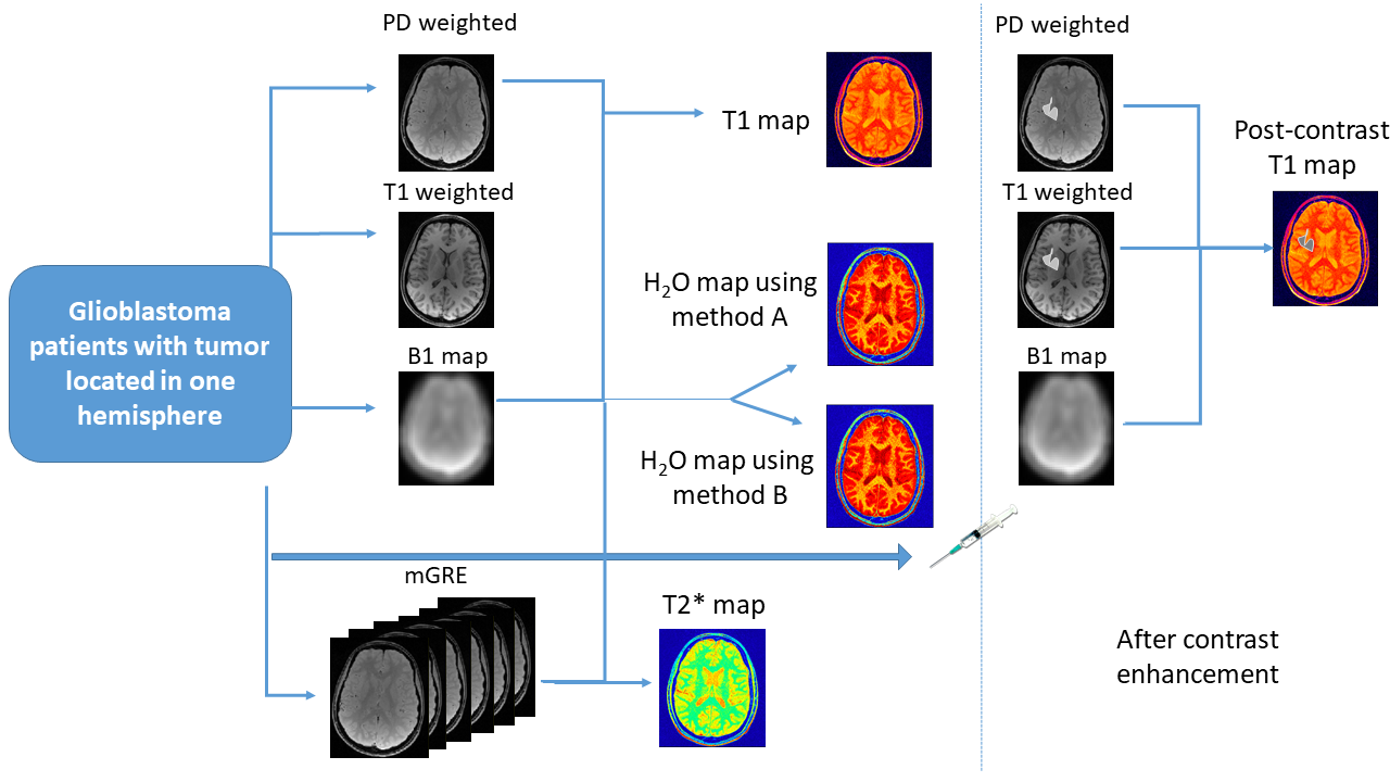
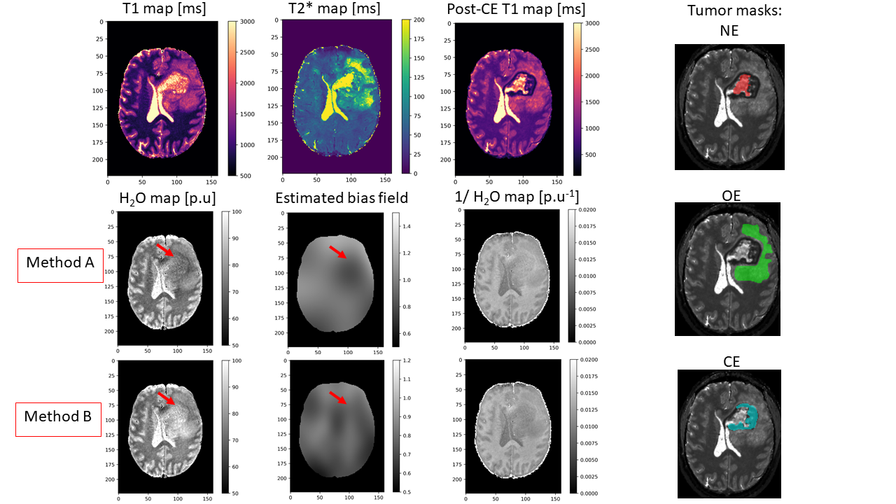
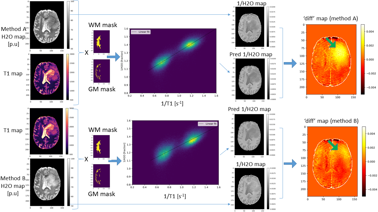
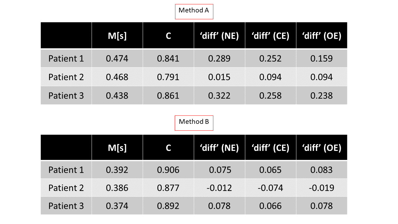
Three patients with IDH-wildtype Glioblastoma (M/49, F/50 and M/72) were scanned with a 3T Magnetom VERIO system, Siemens, Erlangen, Germany. T1 mapping was carried out using the VFA method as in15 (Fig 1), acquiring a PD-weighted and a T1-weighted spoiled gradient echo (GRE) dataset using two different excitation angles (FOV= 256x224x160mm3 matrix size = 256x224x160; TR/TE/α1/α2 = 16.4 ms/6.7 ms/4°/24°; Bandwidth: 222 Hz/pixel, total TA=9min 48sec). B1 mapping was carried out as in16 (identical FoV, 4 mm isotropic resolution, TA=1min). For H2O mapping, the PD weighted image was corrected for the effect of T1, B1, T2* and the bias field. For bias field correction, two approaches were used. Method A: Using a probabilistic framework for tissue segmentation and bias field correction (SPM12)17. Method B: Using a novel method which requires no apriori knowledge, N4ITK18, (weights=0 for tumor tissue, weights=1 for rest of the brain) to avoid the problem of the increased tumor signal compounding the bias field estimation. The bias field was thus estimated outside the tumor tissue and subsequently extrapolated across the whole brain as in19. The predicted 1/H2O maps were computed for the whole brain (using ‘M’ and ‘C’ values obtained from linear regression of WM and GM voxels in the contralateral hemisphere), according to: $$\text { Predicted } \frac{1}{H 2 O}=\frac{M}{T 1}+C$$The difference maps followed from: $$\text { diff }=\frac{1}{H 2 O}-\text { Predicted } \frac{1}{H 2 O}$$Results
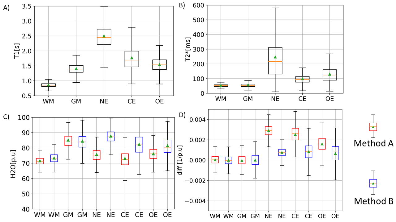
Fig. 2 shows quantitative maps obtained on a representative patient. T1 and T2* maps show a relatively good contrast between the necrotic (NE), oedematous (OE) and contrast enhancing (CE) areas. H2O maps on the other hand show a diffuse change across these areas and depend on the bias field correction method used. Method A induces artificially low H2O values in the tumor region, as described in19. This effect is reduced when Method B is used. In Fig.3, the 2D histograms show an excellent correlation between 1/T1 and 1/H2O in the healthy contralateral hemisphere (‘M’ and ‘C’ values in Table 1). The ‘diff’ maps using Method A show high values in the tumor region, primarily due to the erroneous H2O values obtained with this method. Using method B, this effect is reduced, leading to much lower ‘diff’ values in the tumour region. In Fig. 4, T1 and T2* are seen to be elevated in NE, OE and ST tissues. However, H2O values obtained using either method fail to show a clear difference between tumor tissues and healthy brain tissue, suggesting a decreased diagnostic potential of H2O mapping, per se. However, elevated ‘diff’ values in tumor regions can also be observed with Method B.Discussion and Conclusions
Glioblastoma leads to a local increase in water content and a concomitant increase in T1 and T2* values, as also observed in our study. Concerning the relation between H2O and T1, the significance of ‘diff’ can be interpreted as follows: A linear fit between 1/T1 and 1/H2O in the contralateral healthy hemisphere allows to obtain values for ‘M’ and ‘C’ and thus to predict 1/H2O maps from 1/T1 maps. The good correlation between 1/T1 and 1/H2O is evident in the very low ‘diff’ values in the contralateral hemisphere. In tumor regions, the increase in T1 is a result of (i) increase in H2O and (ii) loss of the short T1 component (e.g. arising from myelin water). Hence, in tumor areas, T1 increases are more pronounced than what one might expect from the H2O increase, yielding lower values of the predicted 1/H2O than the ‘true’ 1/H2O and thus positive ‘diff’ values in tumor regions. In conclusion, the detected minute derangements of the relationship between 1/T1 and 1/H2O in tumor areas and the resulting ‘diff’ maps could potentially provide a new indirect marker of derangements of the microstructure in glioblastomas. Accurate bias field correction techniques are paramount to the success of the method proposed here, as can be seen from the deviation between ‘diff’ values obtained using Method A and Method B.Acknowledgements
KJW and SA were funded by the Mildred Scheel Career Center Frankfurt (Deutsche Krebshilfe). In addition, KJW and DCT were funded by the Else Kröner-Fresenius-Stiftung (EKFS).References
1. B. M. Ellingson et al., “Consensus recommendations for a standardized Brain Tumor Imaging Protocol in clinical trials,” Neuro-Oncol., vol. 17, no. 9, pp. 1188–1198, Sep. 2015, doi: 10.1093/neuonc/nov095.
2. Q. T. Ostrom et al., “The epidemiology of glioma in adults: a ‘state of the science’ review,” Neuro-Oncol., vol. 16, no. 7, pp. 896–913, Jul. 2014, doi: 10.1093/neuonc/nou087.
3. D. R. Johnson and B. P. O’Neill, “Glioblastoma survival in the United States before and during the temozolomide era,” J. Neurooncol., vol. 107, no. 2, pp. 359–364, Apr. 2012, doi: 10.1007/s11060-011-0749-4.
4. U. Nöth, J. Tichy, S. Tritt, O. Bähr, R. Deichmann, and E. Hattingen, “Quantitative T1 mapping indicates tumor infiltration beyond the enhancing part of glioblastomas,” NMR Biomed., vol. 33, no. 3, p. e4242, 2020, doi: 10.1002/nbm.4242.
5. A. Jurcoane et al., “Within-lesion differences in quantitative MRI parameters predict contrast enhancement in multiple sclerosis,” J. Magn. Reson. Imaging, vol. 38, no. 6, pp. 1454–1461, 2013, doi: 10.1002/jmri.24107.
6. G. D. Maurer et al., “Matching Quantitative MRI Parameters with Histological Features of Treatment-Naïve IDH Wild-Type Glioma,” Cancers, vol. 13, no. 16, p. 4060, Aug. 2021, doi: 10.3390/cancers13164060.
7. S. Lescher, A. Jurcoane, A. Veit, O. Bähr, R. Deichmann, and E. Hattingen, “Quantitative T1 and T2 mapping in recurrent glioblastomas under bevacizumab: earlier detection of tumor progression compared to conventional MRI,” Neuroradiology, vol. 57, no. 1, pp. 11–20, Jan. 2015, doi: 10.1007/s00234-014-1445-9.
8. C. Badve et al., “MR Fingerprinting of Adult Brain Tumors: Initial Experience,” Am. J. Neuroradiol., vol. 38, no. 3, pp. 492–499, Mar. 2017, doi: 10.3174/ajnr.A5035.
9. I. Blystad, J. B. M. Warntjes, Ö. Smedby, P. Lundberg, E.-M. Larsson, and A. Tisell, “Quantitative MRI using relaxometry in malignant gliomas detects contrast enhancement in peritumoral oedema,” Sci. Rep., vol. 10, no. 1, Art. no. 1, Oct. 2020, doi: 10.1038/s41598-020-75105-6.
10. A. M. Oros-Peusquens, R. Loução, M. Zimmermann, K.-J. Langen, and N. J. Shah, “Methods for molecular imaging of brain tumours in a hybrid MR-PET context: Water content, T2∗, diffusion indices and FET-PET,” Methods, vol. 130, pp. 135–151, Nov. 2017, doi: 10.1016/j.ymeth.2017.07.025.
11. E. Englund, A. Brun, E. M. Larsson, Z. Györffy-Wagner, and B. Persson, “Tumours of the central nervous system. Proton magnetic resonance relaxation times T1 and T2 and histopathologic correlates,” Acta Radiol. Diagn. (Stockh.), vol. 27, no. 6, pp. 653–659, Dec. 1986, doi: 10.1177/028418518602700606.
12. P. P. Fatouros and A. Marmarou, “Use of magnetic resonance imaging for in vivo measurements of water content in human brain: method and normal values,” J. Neurosurg., vol. 90, no. 1, pp. 109–115, Jan. 1999, doi: 10.3171/jns.1999.90.1.0109.
13. P. P. Fatouros, A. Marmarou, K. A. Kraft, S. Inao, and F. P. Schwarz, “In Vivo Brain Water Determination by T1 Measurements: Effect of Total Water Content, Hydration Fraction, and Field Strength,” Magn. Reson. Med., vol. 17, no. 2, pp. 402–413, 1991, doi: 10.1002/mrm.1910170212.
14. N. Gelman, J. R. Ewing, J. M. Gorell, E. M. Spickler, and E. G. Solomon, “Interregional variation of longitudinal relaxation rates in human brain at 3.0 T: Relation to estimated iron and water contents,” Magn. Reson. Med., vol. 45, no. 1, Art. no. 1, 2001, doi: https://doi.org/10.1002/1522-2594(200101)45:1<71::AID-MRM1011>3.0.CO;2-2.
15. U. Nöth, E. Hattingen, O. Bähr, J. Tichy, and R. Deichmann, “Improved visibility of brain tumors in synthetic MP-RAGE anatomies with pure T1 weighting,” NMR Biomed., vol. 28, no. 7, pp. 818–830, 2015, doi: 10.1002/nbm.3324.
16. S. Volz, U. Nöth, A. Rotarska-Jagiela, and R. Deichmann, “A fast B1-mapping method for the correction and normalization of magnetization transfer ratio maps at 3 T,” NeuroImage, vol. 49, no. 4, pp. 3015–3026, Feb. 2010, doi: 10.1016/j.neuroimage.2009.11.054.
17. J. Ashburner and K. J. Friston, “Unified segmentation,” NeuroImage, vol. 26, no. 3, Art. no. 3, Jul. 2005, doi: 10.1016/j.neuroimage.2005.02.018.
18. N. J. Tustison et al., “N4ITK: Improved N3 Bias Correction,” IEEE Trans. Med. Imaging, vol. 29, no. 6, Art. no. 6, Jun. 2010, doi: 10.1109/TMI.2010.2046908.
19. S. Volz, U. Nöth, A. Jurcoane, U. Ziemann, E. Hattingen, and R. Deichmann, “Quantitative proton density mapping: correcting the receiver sensitivity bias via pseudo proton densities,” NeuroImage, vol. 63, no. 1, Art. no. 1, Oct. 2012, doi: 10.1016/j.neuroimage.2012.06.076.
Figures