2035
Practical Correction of Gradient Nonlinearities in Diffusion-Weighted Imaging
Praitayini Kanakaraj1, Leon Y Cai2, Francois Rheault3, Baxter P Rogers4, Adam Anderson2,4, Kurt G Schilling4, and Bennett A Landman1,2,4,5
1Department of Computer Science, Vanderbilt University, Nashville, TN, United States, 2Department of Biomedical Engineering, Vanderbilt University, Nashville, TN, United States, 3Department of Computer Science, Université de Sherbrooke, Sherbrooke, QC, Canada, 4Department of Radiology and Radiological Sciences, Vanderbilt University Medical Center, Nashville, TN, United States, 5Department of Electrical and Computer Engineering, Vanderbilt University, Nashville, TN, United States
1Department of Computer Science, Vanderbilt University, Nashville, TN, United States, 2Department of Biomedical Engineering, Vanderbilt University, Nashville, TN, United States, 3Department of Computer Science, Université de Sherbrooke, Sherbrooke, QC, Canada, 4Department of Radiology and Radiological Sciences, Vanderbilt University Medical Center, Nashville, TN, United States, 5Department of Electrical and Computer Engineering, Vanderbilt University, Nashville, TN, United States
Synopsis
Keywords: Data Processing, Diffusion/other diffusion imaging techniques
Gradient nonlinearity correction is well-established but not straightforward to implement in existing diffusion software packages due to it producing gradient tables that vary by voxel. We propose a simple, practical approach that approximates full correction by: (1) scaling the diffusion signal and (2) resampling the gradient orientations. Our approach results in uniform gradients across the corrected image and provides the key advantage of seamless integration into current diffusion pipelines. The proposed method resulted in negligible differences in multi- compartment indices from the standard voxel-wise empirical correction.INTRODUCTION
In practice, magnetic field gradients are nonlinear given gradient coil designs and engineering constraints. These nonlinearities in magnetic field gradients give rise to spatial image warping1. In diffusion weighted magnetic resonance imaging (DW-MRI), these systematic spatial distortions result in spatially dependent biases in the magnitude and direction of diffusion gradients2-4. Thus, the achieved diffusion weighted (DW) encoding scheme varies from the one given to the scanner as input. Neglecting correction of nonlinearities can impact diffusion scalar metrics5, tractography6, group-wise studies5, and the reproducibility of apparent diffusion coefficient7. Hence, a correction step is important5. However, the state-of-the-art correction technique proposed by Bammer et al.8 has not become standard practice. We observe that integration into pipelines and models is not straightforward due to the voxel-wise varying gradient table that results (Figure 1). Our work bridges this gap with simple and efficient approximation that estimates the desired diffusion signal from the standard voxel-wise gradient table correction. We validate the proposed technique with a multi-compartment neurite orientation dispersion and density imaging (NODDI) model. Our method allows nonlinearity-corrected DW-MRI to be seamlessly integrated in diffusion workflows.METHODS
Data: For this study, five de-identified subjects from the MASiVar dataset9 approved by the Institutional Review Board were used. The subject scans were acquired at b-value of 1000 s/mm2 for 40 directions and b-value of 2000 s/mm2 for 56 directions. They were scanned on a 3T Philips Achieva scanner with gradient strength of 80 mT/m and 200 T/m/s slew-rate. The empirical field maps were obtained from the same scanner. The empirical field maps are used to estimate the nonlinear gradient tensor L(r) as described10 and reported11 by Rogers et al.Pipeline: The raw diffusion data contain the achieved DW-MRI signal reconstructed from the scanner and desired gradients that were provided as scanner parameters. These desired gradients are mapped voxel-wise to the achieved gradients using the L(r) fields by the widely accepted Bammer et al correction technique5,8,12. From the achieved DW-MRI signal and gradients, we approximate the desired signal with desired gradient table with two steps: 1) scaling the signal through gaussian approximation with the square of the length change in b-value (Eq.1,2) which is numerically equivalent to the magnitude change in the gradients, and 2) resampling the angular change via a spherical harmonics basis (Eq.3) which is numerically equivalent to the orientation change in the gradients (Figure 2). The approach assumes these two steps are separable5. The spherical harmonics fit is performed with the unique set of b-vectors for every voxel. The spherical harmonics basis functions described by Tournier et al13 were implemented using the DIPY library14 with no smoothing and the highest possible even order supported given the number of gradient directions. Finally, the desired signal was estimated with the spherical harmonics coefficients and desired (original) gradients (by rewriting Eq.3). Thus, we estimated a signal overcoming voxel-wise differences after correction for gradient nonlinear fields.
The achieved b-value $$$b^\prime$$$ is computed as8: $$b^\prime=b\ \left|g^\prime\right|^2 .....(1)$$
where $$$b$$$ is the desired b-value and $$$g^\prime$$$ is the achieved gradients. Substitute this in Stejskal-Tanner equation, $$S_{scaled}=\ S_o\ {e\ \ }^\frac{ln\ \ \ {\frac{S_i}{S_o}}}{\left|g^\prime\right|^2} .....(2)$$
where $$$S_i$$$ is diffusion signal at the ith acquisition, $$$S_o$$$ is the reference signal, and $$$S_{scaled}$$$ is the scaled diffusion signal. The spherical harmonics coefficient $$$a_l^m$$$ can be expressed as14 $$a_l^m=\ \int_{S}^{\ }f\left(\theta,\phi\right)Y_l^m\ \left(\theta,\phi\right)\ ds .....(3)$$
where $$$l$$$ is the order, $$$m$$$ is the degree, $$$Y_l^m$$$ is spherical harmonics basis function, and $$$\left(\theta,\phi\right)$$$ represents the direction vector in spherical coordinates.
The proposed approximation was performed separately on each shell. We fit a NODDI model for Bammer correction and proposed approximation with University College of London NODDI Toolbox15. The model generate intra-cellular volume fraction (iVF), cerebrospinal fluid (CSF) volume fraction (cVF), and orientation dispersion index (ODI) representations. For the analysis, we used the white-matter and gray-matter mask from FSL16 for iVF and ODI, while for cVF we used the CSF mask from FSL16.
RESULTS
We show the absolute difference between the voxel-wise Bammer correction and the proposed approximation for iVF (Figure 3), cVF (Figure 4), and ODI (Figure 5) for five subjects. The mean absolute difference in all three NODDI scalar metrics are less than 10-2 between the techniques. The Cohen’s d between the voxel-wise correction and proposed approximation was <0.2 for all subjects. This suggests the approximation does not change the DW-MRI information substantively from the standard Bammer correction technique.CONCLUSION
With the emerging generation of MRI scanners17, the integration of a gradient nonlinearity correction step into contemporary diffusion preprocessing platforms has become necessary. In this work, we have proposed a simple approximation for the standard voxel-wise gradient nonlinearities correction in two steps: scaling the signal with the factor of b-value change from achieved to desired via gaussian approximation and resampling the rescaled signal based on b-vector change from achieved to desired via spherical harmonics approximation. We find that the proposed approximation resulted in negligible differences from the standard voxel-wise correction. Using our proposed approximation, the generally accepted voxel-wise gradient nonlinearity correction for diffusion encoding schemes can be easily incorporated with existing diffusion models. The key limitation was the assumption that the gradient field estimates of scanner are known.Acknowledgements
This work was supported by the National Institutes of Health under award numbers R01EB017230, 1K01EB032898 and T32GM007347, and in part by the National Center for Research Resources, Grant UL1 RR024975-01. The content is solely the responsibility of the authors and does not necessarily represent the official views of the NIH.References
1. Newitt DC, Tan ET, Wilmes LJ, et al. Gradient nonlinearity correction to improve apparent diffusion coefficient accuracy and standardization in the american college of radiology imaging network 6698 breast cancer trial. Journal of Magnetic Resonance Imaging. 2015;42(4):908-919. 2. Conturo TE, McKinstry RC, Aronovitz JA, Neil JJ. Diffusion MRI: precision, accuracy and flow effects. NMR in Biomedicine. 1995;8(7):307-332. 3. Bernstein MA, Polzin JA. Method and system for correcting errors in MR images due to regions of gradient non-uniformity for parametric imaging such as quantitative flow analysis. Google Patents; 2000. 4. Bammer R, Markl M, Pelc N, Moseley M. Assessment of spatial gradient field distortion in diffusion-weighted imaging. Proceedings of the International Society for Magnetic Resonance in Medicine, Honolulu, HI. 2002:1172. 5. Mesri HY, David S, Viergever MA, Leemans A. The adverse effect of gradient nonlinearities on diffusion MRI: From voxels to group studies. NeuroImage. 2020;205:116127. 6. Guo F, De Luca A, Parker G, et al. The effect of gradient nonlinearities on fiber orientation estimates from spherical deconvolution of diffusion magnetic resonance imaging data. Human Brain Mapping. 2021;42(2):367-383. 7. Jovicich J, Czanner S, Greve D, et al. Reliability in multi-site structural MRI studies: effects of gradient non-linearity correction on phantom and human data. Neuroimage. 2006;30(2):436-443. 8. Bammer R, Markl M, Barnett A, et al. Analysis and generalized correction of the effect of spatial gradient field distortions in diffusion‐weighted imaging. Magnetic Resonance in Medicine: An Official Journal of the International Society for Magnetic Resonance in Medicine. 2003;50(3):560-569. 9. Cai LY, Yang Q, Kanakaraj P, et al. MASiVar: Multisite, multiscanner, and multisubject acquisitions for studying variability in diffusion weighted MRI. Magnetic resonance in medicine. 2021;86(6):3304-3320. 10. Rogers BP, Blaber J, Newton AT, et al. Phantom-based field maps for gradient nonlinearity correction in diffusion imaging. International Society for Optics and Photonics; 2018:105733N. 11. Hansen CB, Rogers BP, Schilling KG, et al. Empirical field mapping for gradient nonlinearity correction of multi-site diffusion weighted MRI. Magnetic Resonance Imaging. 2021;76:69-78. 12. Rudrapatna U, Parker GD, Roberts J, Jones DK. A comparative study of gradient nonlinearity correction strategies for processing diffusion data obtained with ultra‐strong gradient MRI scanners. Magnetic Resonance in Medicine. 2021;85(2):1104-1113. 13. Tournier J-D, Calamante F, Connelly A. Robust determination of the fibre orientation distribution in diffusion MRI: non-negativity constrained super-resolved spherical deconvolution. Neuroimage. 2007;35(4):1459-1472. 14. Garyfallidis E, Brett M, Amirbekian B, et al. Dipy, a library for the analysis of diffusion MRI data. Frontiers in neuroinformatics. 2014;8:8. 15. Zhang H, Schneider T, Wheeler-Kingshott CA, Alexander DC. NODDI: practical in vivo neurite orientation dispersion and density imaging of the human brain. Neuroimage. 2012;61(4):1000-1016. 16. Jenkinson M, Beckmann CF, Behrens TE, Woolrich MW, Smith SM. Fsl. Neuroimage. 2012;62(2):782-790. 17. Jones DK, Alexander DC, Bowtell R, et al. Microstructural imaging of the human brain with a ‘super-scanner’: 10 key advantages of ultra-strong gradients for diffusion MRI. NeuroImage. 2018;182:8-38.Figures
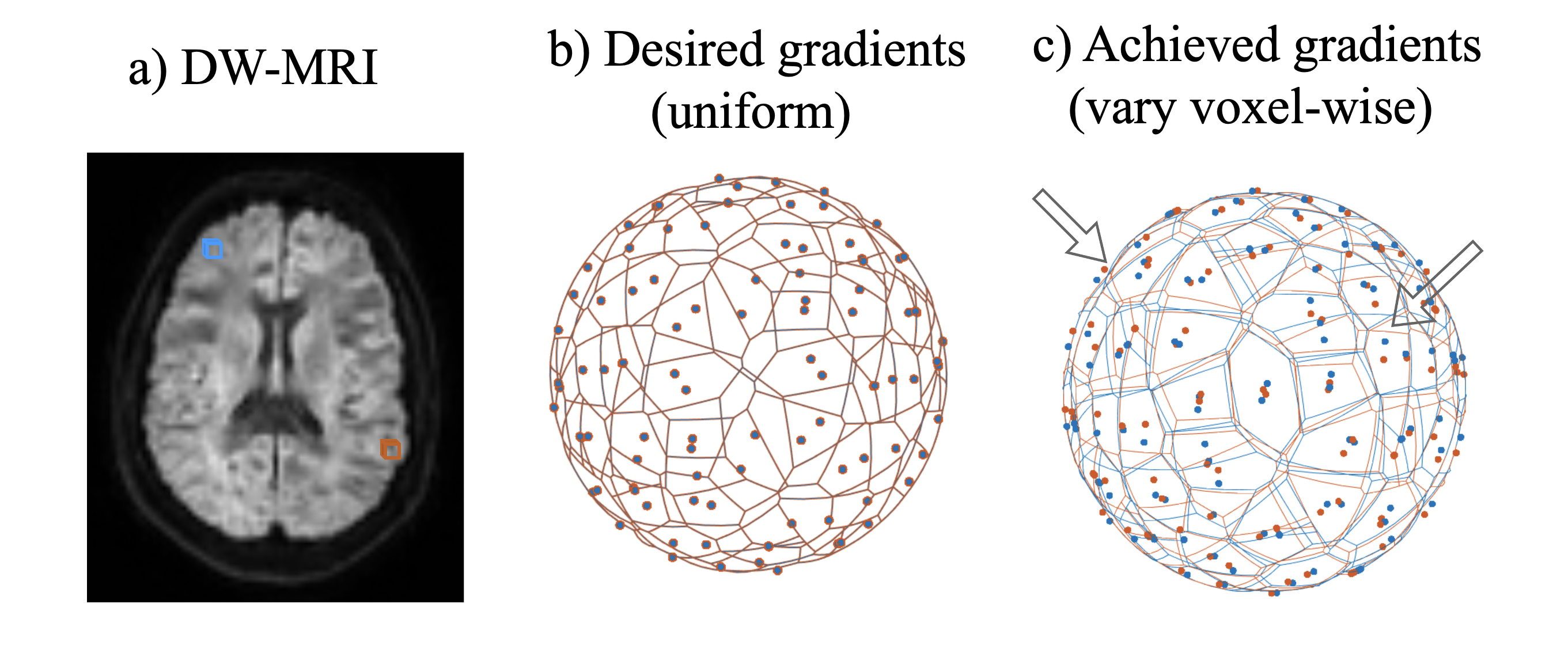
Diffusion MRI (a) pipelines are set up to take 3D
dimensional space and intersect it conditionally in a 3D space with uniform desired
magnitude and orientation of the gradients (b) (shown for two voxels
highlighted in blue and red in (a)) . However, the magnitude and orientation of
the achieved gradients vary by voxel (c) with the Bammer gradient nonlinearities
correction. Note, the arrows point to the
variations in orientation of gradients between the blue and red voxels. It
would require modification of existing diffusion pipelines to use these
voxel-wise magnitude and orientation.
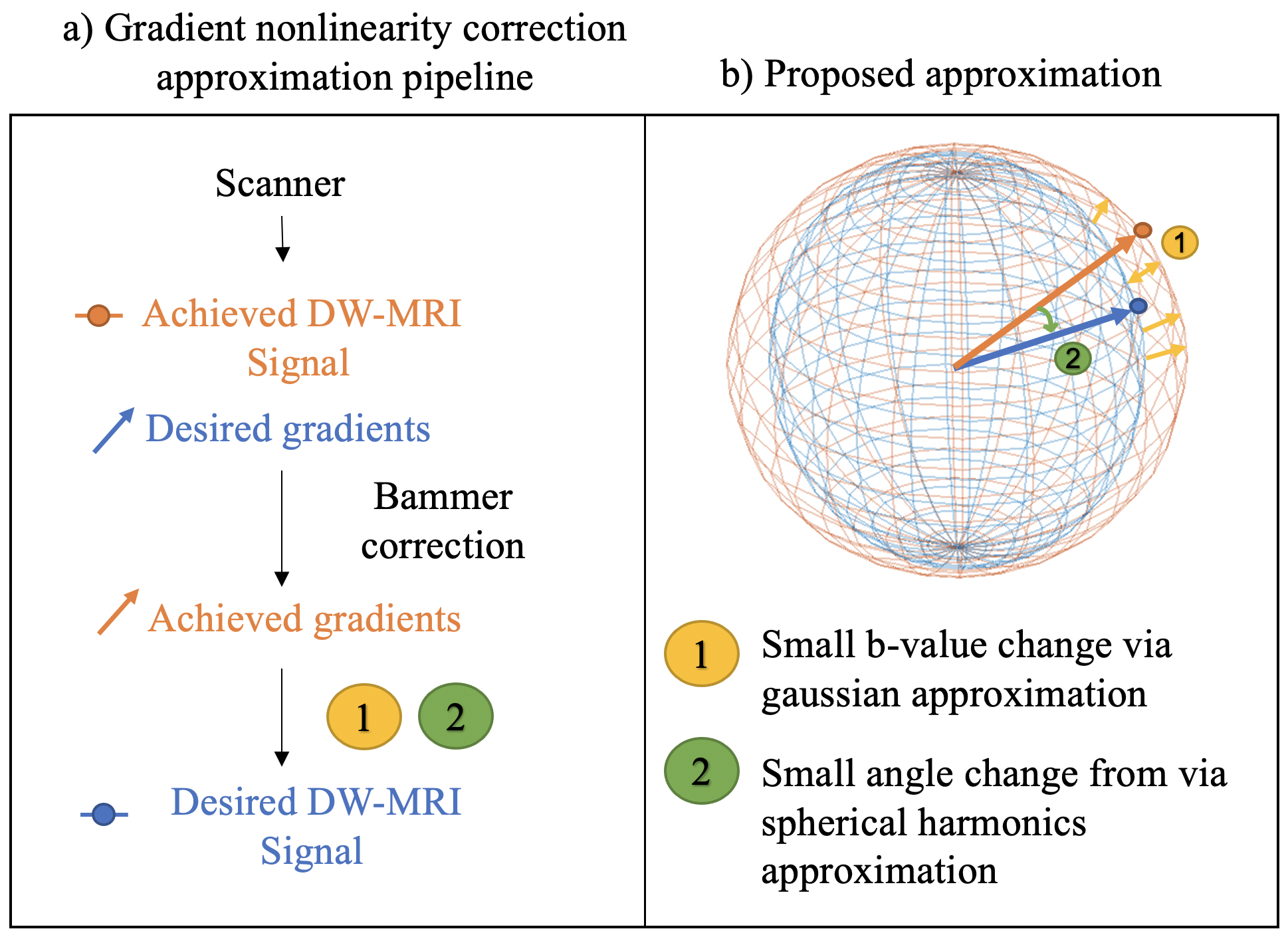
The
(a) pipeline and (b) idea of the proposed approximation. a) From the scanner we get
the achieved DW-MRI signal and desired gradients given as scanner parameters.
After Bammer correction, we obtain the achieved gradients for each voxel. (b) From
the achieved gradients we approximate the desired signal by 1) reshaping the
sphere by rescaling the signal based on b-value change from achieved to desired
via gaussian approximation and 2) rotating the sphere by resampling the
rescaled signal based on b-vector change from achieved to desired via spherical
harmonics approximation.
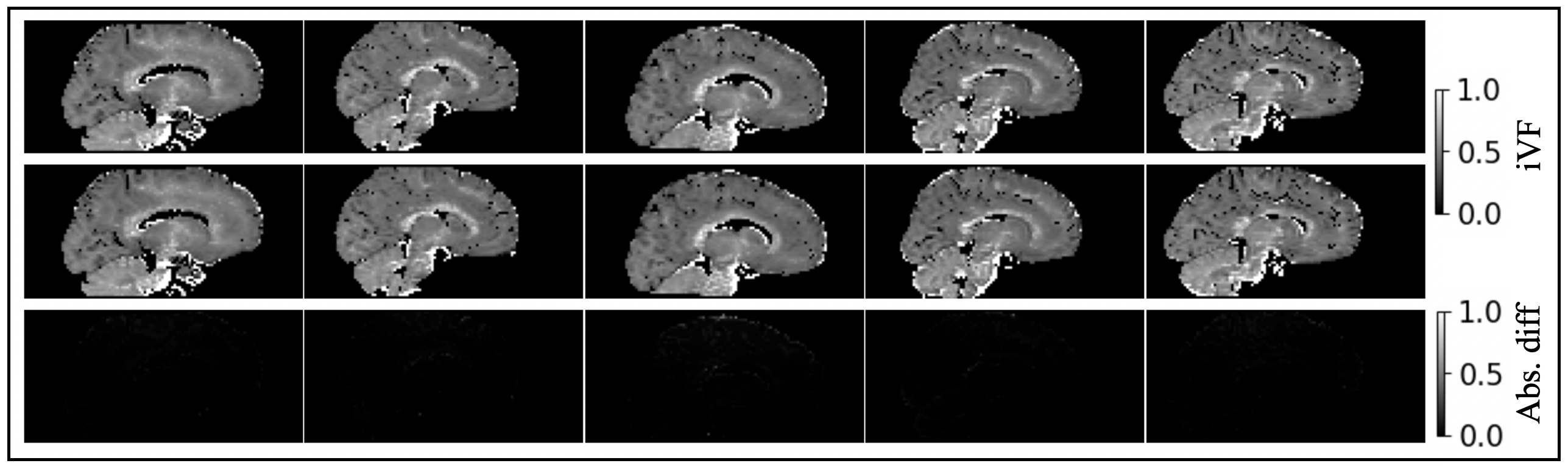
Validation of proposed approximation
in
intra-cellular volume fraction (iVF). Each column represents one subject. The iVF after
voxel-wise gradient nonlinearity correction are shown in the first row of each
panel. The iVF after the proposed approximation are shown in the second
row.
The absolute difference between the two are shown in the
third row of each panel. The absolute difference of the scalar maps are near
zero.
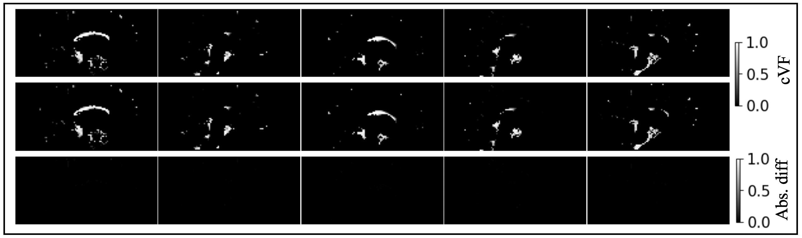
Validation of proposed approximation
in
cerebrospinal fluid volume fraction (cVF). Each column represents one subject. The cVF after
voxel-wise gradient nonlinearity correction are shown in the first row of each
panel. The cVF after the proposed approximation are shown in the second
row.
The absolute difference between the two are shown in the
third row of each panel. The absolute difference of the scalar maps are near
zero.
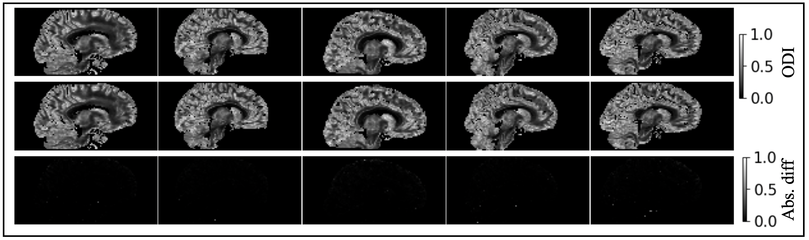
Validation of proposed approximation
in
orientation dispersion index (ODI). Each column represents one subject. The ODI after
voxel-wise gradient nonlinearity correction are shown in the first row of each
panel. The ODI after the proposed approximation are shown in the second
row.
The absolute difference between the two are shown in the
third row of each panel. The absolute difference of the scalar maps are near
zero.
DOI: https://doi.org/10.58530/2023/2035