2008
In-plane B0 inhomogeneity effects in T2* mapping
Glen Morrell1
1Radiology and Imaging Sciences, University of Utah, Salt Lake City, UT, United States
1Radiology and Imaging Sciences, University of Utah, Salt Lake City, UT, United States
Synopsis
Keywords: Artifacts, Relaxometry
Main field B0 inhomogeneity may adversely affect the accuracy of T2* mapping in the abdomen even at locations spatially distant from the B0 variation. We show this effect in both simulation and phantom studies, and show that it can be ameliorated with the use of two-dimensional spatially selective excitation. These findings have important ramifications for applications of BOLD imaging in the abdomen such as renal BOLD or liver T2* mapping, where large B0 inhomogeneity is often present in areas of the image volume spatially remote from the organ of interest.Introduction
T2* mapping (BOLD) has found wide application in various parts of the body. Originally developed for functional imaging in the brain, BOLD has subsequently been attempted in various other organs including kidney1 and liver2. The use of BOLD in the abdomen introduces challenges not present in brain imaging, including a potential wide range of B0 homogeneity across the image volume, including inhomogeneity near the edges of the body caused by magnet design and large susceptibility shifts at interfaces such as the lung and diaphragm or air-filled bowel loops. The effects of through-slice B0 inhomogeneity within or near the target organ on T2* mapping has been studied3. In-plane B0 inhomogeneity has typically been neglected. We show with numerical simulation and phantom studies that in-plane B0 inhomogeneity may cause significant inaccuracy in T2* maps even when the area of inhomogeneity is spatially distant from the organ of interest. We also demonstrate the use of 2D spatially selective excitation to ameliorate these effects.Theory
The 3D voxel sensitivity function (VSF) resulting from Fourier transform reconstruction of a Cartesian k-space is given by4 $$vsf(x,y,z) = \frac{1}{N_xN_yN_z} \frac{\sin(\pi \frac{x}{\Delta x}) \sin(\pi \frac{y}{\Delta y}) \sin(\pi \frac{z}{\Delta z})}{\sin(\pi \frac{x}{N_x \Delta x}) \sin(\pi \frac{y}{N_y \Delta y}) \sin(\pi \frac{z}{N_z \Delta z})}$$.The function vsf(x,y,z) has a large central sinc-like lobe and sidelobes of alternating sign spaced at the pixel spacing of the image. Unlike the sinc function, the voxel sensitivity function does not fall off as quickly with distance from the origin. This creates the opportunity for signal from spatially remote regions to contribute substantially to the value of a given image pixel. This is usually not of practical concern because the alternating positive and negative oscillations of the vsf tend to cancel, and we typically think of the image as representing the convolution of just the central sinc-like lobe of the VSF with the actual signal distribution m(x,y,z). However, this assumption may be faulty in situations where a phase gradient exists over portions of the object which is of appropriate amplitude to effectively invert the sign of every other lobe of the VSF, causing these lobes to add and potentially contribute significant signal to a pixel spatially remote from the phase gradient.
Methods
We performed a numerical simulation of the evolution of the MRI signal in two dimensions using a synthetic B0 map with exponential variation of B0 near the edge of a theoretical object. Simulation was performed over a grid with ten times the in-plane voxel resolution, and the resulting image pixel value was obtained for each point in time by summing the individual simulation grid points multiplied by the VSF. Figure 1 shows the B0 map and the signal evolution with echo time for a single point from the 2D image plane.A phantom study was performed by taping a paperclip to the side of a liquid phantom, creating B0 inhomogeneity at the edge of the image volume. A 3D multi-echo GRE sequence was then used with a series of echo times (1, 6, 11, 16, 21, 26, 31, 36, 41, and 46 msec). The sequence was then repeated five times with the echo times incremented by 1 msec each time, yielding a complete data set of images from echo times from 1 to 50 msec at 1 msec increments. The experimental B0 map and a representative 1 msec echo time image are shown in Figure 2, along with the measured signal evolution at a single point in the image volume.
Additional phantom imaging was then performed using a 2D spatially selective excitation pulse which excited a cylinder within the image plane shown in Figure 2. The signal evolution with echo time for the 2D excitation is also shown in Figure 2.
Results
Simulation (Figure 1) shows wide variation in the signal intensity at a point distant from the B0 inhomogeneity. The B0 inhomogeneity at the left of the volume causes the signal evolution from points in the right of the volume to vary from the expected monoexponential decay. This result is verified in the phantom study shown in Figure 2, where B0 inhomogeneity at one edge of the image volume causes significant deviation of the signal evolution from the expected monoexponential decay even at points spatially distant from the B0 inhomogeneity. If 2D spatially selective excitation is used, the variation in signal intensity is ameliorated, as shown in Figure 2.Conclusion
We have demonstrated that B0 inhomogeneity spatially distant from the organ of interest can cause significant deviation of the signal evolution from the expected monoexponential decay upon which T2* mapping relies. Depending on the choice of echo times used for a particular T2* mapping experiment, this deviation of signal intensity may introduce large errors in T2* estimation. This effect can be overcome with spatially selective excitation, which excludes signal from the spatially distant areas of B0 inhomogeneity. This observation may have important clinical application in settings such as renal BOLD MRI, where the image volume typically includes areas of significant B0 inhomogeneity such as the edges of the body and air-tissue interfaces such as lung and bowel.Acknowledgements
No acknowledgement found.References
1. Prasad PV, Edelman RR, Epstein FH. Noninvasive evaluation of intrarenal oxygenation with BOLD MRI. Circulation 1996;94(12):3271-3275.
2. Hernando D, Levin YS, Sirlin CB, Reeder SB. Quantification of liver iron with MRI: state of the art and remaining challenges. J Magn Reson Imaging 2014;40(5):1003-1021.
3. Hernando D, Vigen KK, Shimakawa A, Reeder SB. R*(2) mapping in the presence of macroscopic B(0) field variations. Magn Reson Med 2012;68(3):830-840.
4. Parker DL, Du YP, Davis WL. The voxel sensitivity function in Fourier transform imaging: applications to magnetic resonance angiography. Magn Reson Med 1995;33(2):156-162.
Figures
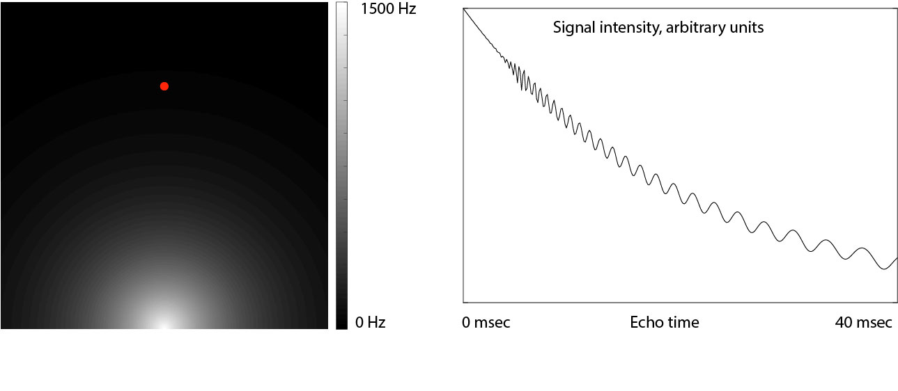
Simulation results: An object of uniform proton density was simulated in a 2D image plane with the B0 map shown on the left, which has exponentially varying inhomogeneity. The evolution of signal with echo time observed at a single point distant from the B0 inhomogeneity designated by the red dot is plotted. Actual T2* was specified as 40 msec. The time evolution of signal with echo time deviates from the expected monoexponential decay because the B0 inhomogeneity even at points spatially remote from the inhomogeneity.
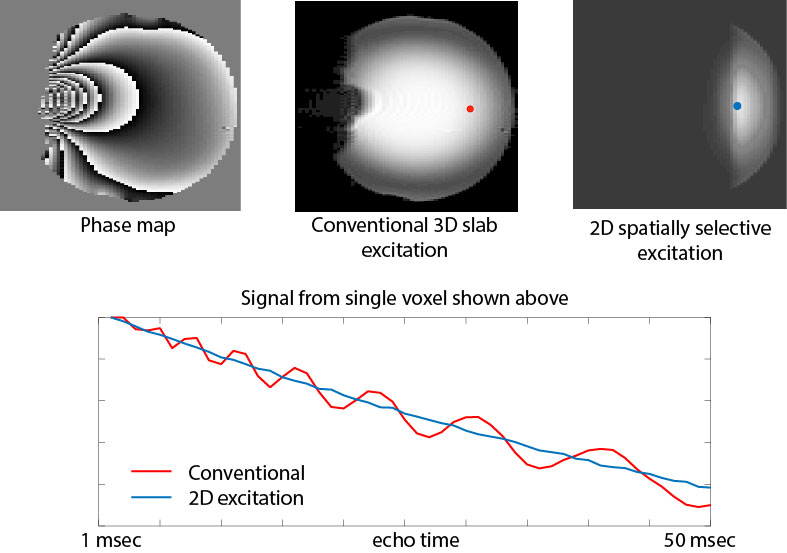
Phantom results: An axial slice from a 3D GRE scan of a spherical phantom with a range of echo times from 1 to 50 msec. A paperclip was taped to the side of the phantom, producing B0 inhomogeneity reflected in the phase map. The evolution of signal intensity with echo time is shown for a single point in the 3D volume spatially distant from the paper clip. The experiment was repeated with a spatially selective 2D excitation (right panel) which excites the area of interest but does not excite the areas of worst B0 inhomogeneity, restoring the expected smooth exponential signal decay.
DOI: https://doi.org/10.58530/2023/2008