1883
Biparametric MRI classification model for prostate cancer detection using a combination of prediction maps
Mohammed R. S. Sunoqrot1,2, Rebecca Segre1,3, Gabriel A. Nketiah1,2, Alexandros Patsanis1, Tone F. Bathen1,2, and Mattijs Elschot1,2
1Department of Circulation and Medical Imaging, Norwegian University of Science and Technology (NTNU), Trondheim, Norway, 2Department of Radiology and Nuclear Medicine, St. Olavs Hospital, Trondheim University Hospital, Trondheim, Norway, 3Department of Mechanical and Aerospace Engineering, Politecnico di Torino, Torino, Italy
1Department of Circulation and Medical Imaging, Norwegian University of Science and Technology (NTNU), Trondheim, Norway, 2Department of Radiology and Nuclear Medicine, St. Olavs Hospital, Trondheim University Hospital, Trondheim, Norway, 3Department of Mechanical and Aerospace Engineering, Politecnico di Torino, Torino, Italy
Synopsis
Keywords: Machine Learning/Artificial Intelligence, Prostate
Biparametric MRI (bpMRI) is a valuable tool for the diagnosis of prostate cancer (PCa). Computer-aided detection and diagnosis (CAD) systems have the potential to improve the robustness and efficiency of PCa detection) compared with conventional radiological reading. This work explores the combination of the results of two PCa CAD systems as input to a new classification model. We show that this is promising approach that can potentially improve the final detection of PCa.INTRODUCTION
Biparametric MRI (bpMRI) is an important tool for the diagnosis of prostate cancer (PCa)1,2. bpMRI involves the acquisition of T2-weighted imaging (T2W) and diffusion-weighted imaging (DWI). The apparent diffusion coefficient (ADC)3 can be calculated from DWIs with different b-values4. Currently, bpMR images are interpreted qualitatively by a radiologist, which requires expertise, is time-consuming, and is subject to inter-observer variability5. Computer-aided diagnosis (CAD) systems have been proposed to overcome these limitations5. Two in-house CAD systems were previously developed to generate maps for predicting PCa probability. However, the combination of both models’ outputs has not been investigated. Therefore, the aim of this work was to combine the output of both models using a multichannel 3D convolutional neural network (CNN) to distinguish between patients with clinically significant PCa (csPCa) and patients with non-csPCa.METHODS
DatasetsIn this study, an in-house collected bpMRI dataset (n=504) was used. Images were acquired on MAGNETOM Skyra 3T MR scanner (Siemens Healthineers, Erlangen, Germany), without endorectal coil. T2W images were acquired using a turbo spin-echo sequence and DWI images (0≤b-value≤800) were acquired with a single-shot echo planar sequence. The regional committee for medical and health research ethics approved the use of the dataset (identifier 2017/576). Patients with biopsy findings of Gleason grade group≥2 were considered to have csPCa. The dataset was shuffled and split into training (72%, 182/182 csPCa/non-csPCa), validation (18%, 45/45 csPCa/non-csPCa), and testing set (10%, 25/25 csPCa/non-csPCa).
Workflow
The study workflow is shown in Figure 1. bpMRI images are prepared and pre-processed before they are fed into two CAD systems to produce prediction maps, which are then used as input to a 3D CNN classification model.
Pre-processing: b-value=1500 images and ADC maps were calculated from the DW images using a monoexponential model. Then, DW images were co-registered to the T2W images using elastix (v.5.0.0)6. Automatic segmentation (trained with 89 cases) of the whole prostate was then performed using 3D models (V-Net7 and , nnU-Net8). The best of the two segmentations was selected based on a segmentation quality control system9. The T2W images were normalized using AutoRef10.
Prediction maps: pre-processed images are used as input to two CAD systems:
- The tumor probability map (TPM): The prostate segmentations were used to extract 132 voxel-wise radiomics features (94 intensity and texture, 19 intensity, and 19 intensity features for T2W, DW, and ADC images, respectively) using PyRadiomics (V3.0.1)11 and 5 anatomical features from the T2W images. The features were then fed into an XGBoost classifier trained with 295 cases (199 from PROSTATEx12 and 96 from PCa-MAP13) to generate a 3D tumor probability map showing the probability that a voxel is a csPCa.
- The anomaly score maps (ASM): Here, the images were cropped using the stride technique and fed into a 3-channel Fixed-Point GAN model14 trained with 263 cases from another in-house dataset. The model generates three 3D images representing ‘healthy’ T2W, DW, and ADC images. Each of the images was then post-processed by creating a 3D difference map between the input images and the generated images. The maps were then filtered with local mean to generate a patient-level anomaly score map representing the likelihood of having PCa (defined as grade group≥1).
Performance evaluation
The performance of the classification model was evaluated by running the model 5 times with different initiations, and then calculating the mean and standard deviation (SD) of the area under the ROC curve (AUC). For comparison, the model was trained with TPM only (1 map), ASM only (3 maps), and TPM and ASM combined (4 maps). Student's paired t-test was used to assess statistical differences between AUC values.
RESULTS
Figure 3 shows the ROC curves of the validation and test sets for the run with the highest validation performance. Table 1 shows the performance results for all runs and their mean±SD. The 4-maps model had the highest AUC (mean±SD=0.903±0.005 on the test set). A significant difference (p<0.01) was found between the 4-maps and 3-maps models for the test set.DISCUSSION
Our proposed classification system based on the combination of two fundamentally different CAD systems showed good performance with low variance. This indicates that combining prediction maps and using them as input to a new classification network can improve csPCa classification.The AUC improvement resulting from combining the two CAD systems' maps is not significant compared to using TPM alone. However, the observed improvement at ROC curves indicates that the combination may help to reduce the false-positive and false-negative rates. However, the model needs further investigation, optimization, and evaluation on larger and more diverse dataset.
CONCLUSION
We developed a 3D multichannel CNN model combining 4 prediction maps from 2 CAD systems, which improved the performance of detecting csPCa on bpMRI.Acknowledgements
No acknowledgement found.References
- Turkbey, B. et al. Prostate Imaging Reporting and Data System Version 2.1: 2019 Update of Prostate Imaging Reporting and Data System Version 2. Eur Urol 76, 340-351, doi:10.1016/j.eururo.2019.02.033 (2019).
- Scialpi, M., Aisa, M. C., D'Andrea, A. & Martorana, E. Simplified Prostate Imaging Reporting and Data System for Biparametric Prostate MRI: A Proposal. AJR Am J Roentgenol 211, 379-382, doi:10.2214/AJR.17.19014 (2018).
- Westbrook, C., Roth, C. K. & Talbot, J. MRI in practice. 4th edn, (Wiley-Blackwell, 2011).
- Stabile, A. et al. Multiparametric MRI for prostate cancer diagnosis: current status and future directions. Nat Rev Urol 17, 41-61, doi:10.1038/s41585-019-0212-4 (2020).
- Lemaitre, G. et al. Computer-Aided Detection and diagnosis for prostate cancer based on mono and multi-parametric MRI: a review. Comput Biol Med 60, 8-31, doi:10.1016/j.compbiomed.2015.02.009 (2015).
- Klein, S., Staring, M., Murphy, K., Viergever, M. A. & Pluim, J. P. W. elastix: A Toolbox for Intensity-Based Medical Image Registration. Ieee Transactions on Medical Imaging 29, 196-205, doi:10.1109/Tmi.2009.2035616 (2010).
- Milletari, F., Navab, N. & Ahmadi, S. A. V-Net: Fully Convolutional Neural Networks for Volumetric Medical Image Segmentation. Int Conf 3d Vision, 565-571, doi:10.1109/3dv.2016.79 (2016).
- Isensee, F., Jaeger, P. F., Kohl, S. A. A., Petersen, J. & Maier-Hein, K. H. nnU-Net: a self-configuring method for deep learning-based biomedical image segmentation. Nat Methods, doi:10.1038/s41592-020-01008-z (2020).
- Sunoqrot, M. R. S. et al. A Quality Control System for Automated Prostate Segmentation on T2-Weighted MRI. Diagnostics (Basel) 10, doi:10.3390/diagnostics10090714 (2020).
- Sunoqrot, M. R. S., Nketiah, G. A., Selnaes, K. M., Bathen, T. F. & Elschot, M. Automated reference tissue normalization of T2-weighted MR images of the prostate using object recognition. Magn Reson Mater Phy 34, 309-321, doi:10.1007/s10334-020-00871-3 (2021).
- van Griethuysen, J. J. M. et al. Computational Radiomics System to Decode the Radiographic Phenotype. Cancer Res 77, e104-e107, doi:10.1158/0008-5472.CAN-17-0339 (2017).
- Armato, S. G., 3rd et al. PROSTATEx Challenges for computerized classification of prostate lesions from multiparametric magnetic resonance images. J Med Imaging (Bellingham) 5, 044501, doi:10.1117/1.JMI.5.4.044501 (2018).
- Maas, M. C. et al. A Single-Arm, Multicenter Validation Study of Prostate Cancer Localization and Aggressiveness With a Quantitative Multiparametric Magnetic Resonance Imaging Approach. Invest Radiol 54, 437-447, doi:10.1097/RLI.0000000000000558 (2019).
- Siddiquee, M. M. R. et al. Learning Fixed Points in Generative Adversarial Networks: From Image-to-Image Translation to Disease Detection and Localization. Proc IEEE Int Conf Comput Vis 2019, 191-200, doi:10.1109/iccv.2019.00028 (2019).
Figures
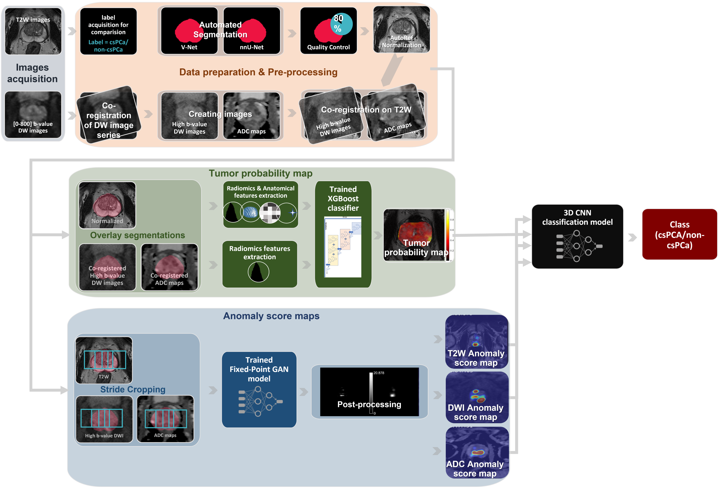
Figure 1: The study
workflow starts with the creation of the high b-value DW images and the ADC
maps. The T2W images are normalized, and all other images are co-registered to
them. Automatic segmentation of the whole prostate is then performed using two
3D deep learning systems, and the segmentation quality control system selects
the best masks. The images are then used as input to two systems to generate a
tumour probability map and 3 anomaly score maps. The 4 maps are then used as
input to a 3D CNN classification model to perform patient-level classification.
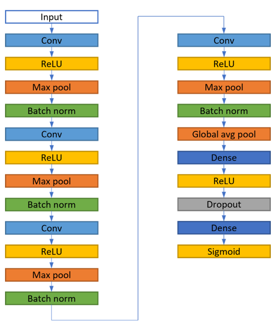
Figure 2: The structure
of the 3D classification model of the convolutional neural network (CNN). The
model takes 4 channels with a size of 64×64×32 as input and provides one class
as output. The model was trained with a learning rate of 10-5 and
batch size of 32. The cross-entropy loss function and stochastic gradient
descent optimizer were used. The model was implemented with Tensorflow Keras
API (v.2.9.0) using Python (v.3.9.12) on an NVIDIA Tesla P100 PCle 16 GB GPU
Ubuntu 18.04.6 LTS.
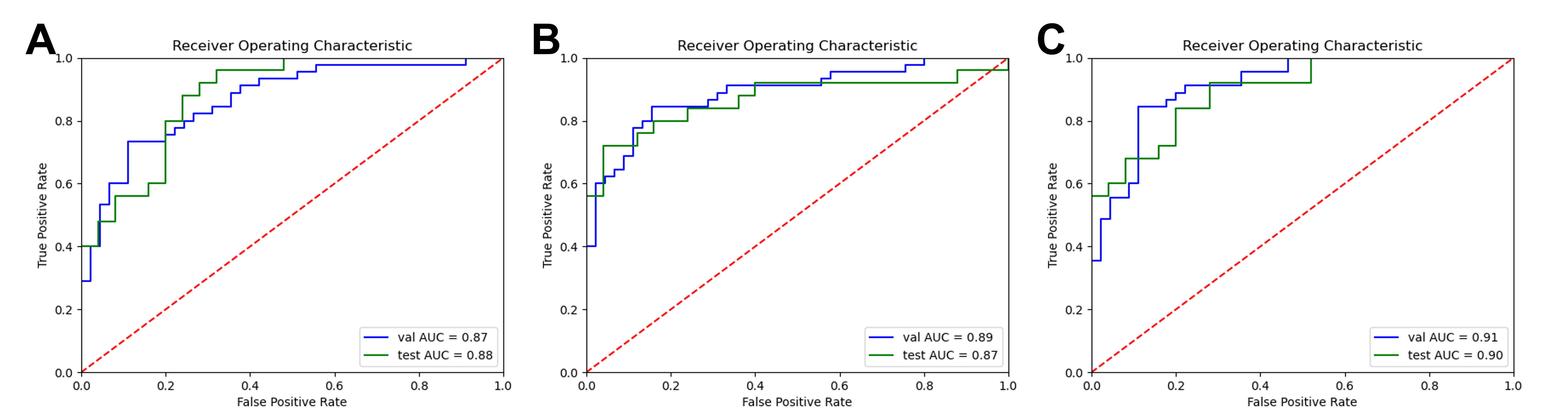
Figure 3: Receiver
operation characteristic (ROC) curves for the model run with the best
performance on the validation set when the classification model was trained
with (A) TPM only (1 map), (B) the ASM only (3 maps), and (C) TPM and ASM
combined (4 maps). The highest AUC values were obtained by the model trained
with the combined 4 maps (AUC = 0.91, and 0.90 for the validation, and test
sets, respectively).
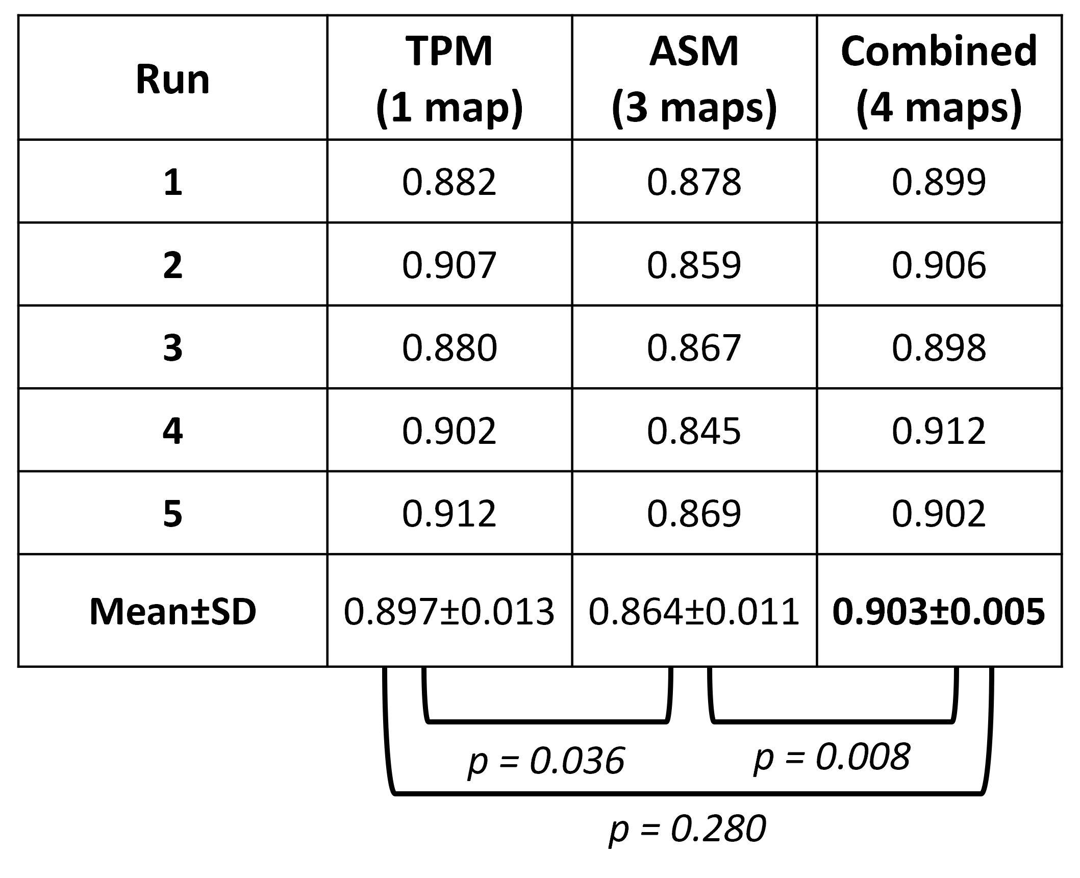
Table 1: The area under
the receiver operation characteristic curves (AUC) for the classification model
at 5 runs on the test set when trained with TPM only (1 map), ASM only (3
maps), and TPM and ASM combined (4 maps), and their mean and standard deviation
(SD). In addition to the results of the statistical differences between AUC
values.
DOI: https://doi.org/10.58530/2023/1883