1875
Primary prostate cancer characterisation using internal references for 23Na MRI quantification1Computer Assisted Clinical Medicine, Medical Faculty Mannheim, Heidelberg University, Mannheim, Germany, 2Mannheim Institute for Intelligent Systems in Medicine, Medical Faculty Mannheim, Heidelberg University, Mannheim, Germany, 3Department of Radiology and Nuclear Medicine, Mannheim University Medical Centre, Mannheim, Germany, 4Department of Urology and Urosurgery, Mannheim University Medical Centre, Mannheim, Germany, 5Department of Radiology, Kantonsspital Baden, Baden, Switzerland
Synopsis
Keywords: Prostate, Tumor
Aim of this prospective study was to evaluate 23Na MRI of 36 patients with suspected prostate cancer and quantify tissue sodium concentration (TSC) based on internal references. TSC reference regions were defined within both femoral blood vessels (FBV), where TSC showed no significant differences between both sides (3.3±2.2 mM, p=0.076). TSC in the prostate was 39.0±5.3 mM; significantly higher in the peripheral than in the transitional zone (p=0.0004, mean difference 4.7±3.5 mM). Nine lesions were segmented and showed mean TSC of 32.2±5.5, significantly lower than contralateral (p=0.0181). TSC might represent a quantitative biomarker that could improve prostate lesion characterization.Introduction
Multiparametric MRI (mpMRI) protocols as defined by the Prostate Imaging-Reporting and Data System (PI-RADS) guidelines aim for the detection and characterisation of prostate carcinoma (PCa) (1, 2, 3). However, specificity of mpMRI remains limited (4). Tissue sodium concentration (TSC) from 23Na MRI offers information about cellular integrity (5) and previous studies have found altered sodium levels in PCa (6-10) implying that TSC might be able to improve characterisation of prostate lesions. Quantitative 23Na MRI requires references with a known sodium concentration. External reference phantoms are considered state-of-the-art (11) but quantification accuracy is impaired by field and coil inhomogeneities, which is affected by distance between reference and region of interest (ROI). Alternatively, internal references in spatial proximity to the ROI (12,13) could be used, which might reduce such impact. Specifically, femoral blood vessels (FBV) are well distinguishable on prostate images and could serve as references. The aim of this study was to evaluate 23Na MR images of prostate cancer and quantify TSC based on internal references.Materials and Methods
The data of thirty-six patients (mean age: 66.5±7.5 years) with clinically suspected prostate cancer was analysed in a prospective IRB approved study. Patients underwent clinical mpMRI and an additional 23Na MRI examination. Imaging was performed at 3T (Magnetom Skyra, Siemens Healthineers, Erlangen, Germany) and a dual-tuned 1H/23Na body-coil (Rapid Biomedical, Rimpar, Germany) was used to acquire the 3D radial density-adapted 23Na sequence (TR/TE=120/1.2 ms, 8,000 spokes, slew rate 170 T/s m, bandwidth 50 Hz/px, acquisition time 16 min) (14). PI-RADS scores were defined for each patient and segmentation of the whole prostate (WP), its peripheral zone (PZ), suspicious lesions (PI-RADS 4 and 5) and contralaterally mirrored lesions were performed in MITK (German Cancer Research Center, Heidelberg, Germany). 23Na MR image reconstruction and co-registration was performed in MATLAB 2018a (The Mathworks Inc., Nattick, USA). After image reconstruction of each of the coil’s 16 receive channels, they were combined via adaptive coil combination (ACC) (15). Inhomogeneities of the coil's receive field (B1-) were corrected by applying a low-pass filter (Gaussian filter) to the 23Na image ($$$NaIm$$$) (𝜎1=10 voxels, filter size = 41 voxels) (Figure 1). The method was similar to the publication by Lachner et al. (16). A binary mask was obtained by thresholding. A second Gaussian filter was applied to the mask (𝜎2=20 voxels, filter size = 81 voxels), allowing calculation of the B1- correction map $$$B1^-_{corr}$$$, based on which the B1--corrected image ($$$NaB1^-_{corr}$$$) was obtained with:$$NaB1^-_{corr}=\frac{NaIm}{B1^-_{corr}}$$
For TSC quantification, ROIs were defined within the right and left FBV (Figure 2). Previously reported TSC levels in the blood were around 81 mM (17-19), which was assumed within the FBV. Relaxation time corrections were performed in blood and prostate tissue. Mean TSC was calculated within WP, PZ, transitional zone (TZ), lesions and contralateral ROIs (Figure 3). SD of TSC within both FBV and absolute TSC differences between right and left FBV were considered to evaluate reproducibility and stability of the method. The student t-test was used to evaluate whether TSC differences (between both sides of the FBV and between PCa lesions and contralateral ROIs) were statistically significant, which was applicable as TSC followed normal distribution.
Results
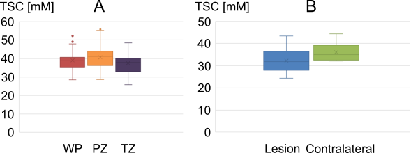
The patients were rated with PI-RADS 5 (n=5), PI-RADS 4 (n=3) , or with lower ranking lesions (n=28). All patients with suspicious lesions had biopsy-proven PCa with Gleason ≥ 3+3. TSC in the ROIs within the FBV showed no significant differences between both sides (3.3±2.2 mM, p=0.076). Mean SD was 3.2±1.3 mM (left) and 3.9 ± 1.7 mM (right). Within the WP, mean TSC was 39.0 ± 5.3 mM. In the PZ, it was with 40.7±6.0 mM significantly higher than in the TZ 37.5±5.7 mM (p=0.0004, mean difference 4.7 ± 3.5 mM). Nine lesions (from eight patients) were segmented and showed a mean TSC of 32.2 ± 5.5, whereas mean TSC in the contralateral ROIs was with 36.1±3.9 significantly lower (p=0.0181) (Table 1, Figure 4).Discussion
This prospective study confirmed that usage of internal references is a feasible technique for quantifying TSC of prostate tissue and suspicious lesions. Significantly reduced TSC was found within PCa lesions. TSC quantification using external reference phantoms carries hazards because of B1 inhomogeneities and greater distances between references and ROIs. FBV as reference reduces those inaccuracies but introduces additional confounders like the patient's blood sodium concentration and hematocrit levels (20). Differences between TSC in the right and left FBV were not significant, indicating sufficient stability of the quantification method. Observed TSC in prostate tissue was similar to previously reported values (6-10). This study showed mean TSC levels in PZ to be significantly higher than TSC in TZ, which was also found in previous studies. TSC in PCa lesions was significantly lower than TSC in the contralateral ROIs (healthy tissue), which is opposite to previous studies. Barret et al. and Broeke et al. reported elevated TSC in PCa (6-8). In tumors, an increased cell metabolism and vascularisation might increase intracellular sodium concentration and relative extracellular volume. However, tumors’ higher cell density also decreases extracellular volume fraction, which might explain the decreased TSC in PCa lesions.Conclusion
TSC might represent a non-invasive, quantitative biomarker that could improve prostate lesion characterisation.Acknowledgements
This research project is part of the Research Campus M2OLIE and funded by the German Federal Ministry of Education and Research (BMBF) within the Framework “Forschungscampus: public-private partnership for Innovations” under the funding code 13GW0388A and 13GW0092D.References
1. Dickinson L, Ahmed HU, Allen C, et al. Magnetic resonance imaging for the detection, localisation, and characterisation of prostate cancer: recommendations from a European consensus meeting. European urology. 2011;59(4):477-94.
2. Gupta RT, Spilseth B, Patel N, et al. Multiparametric prostate MRI: focus on T2-weighted imaging and role in staging of prostate cancer. Abdominal Radiology. 2016;41(5):831-43.
3. Kurhanewicz J, Vigneron D, Carroll P, Coakley F. Multiparametric magnetic resonance imaging in prostate cancer: present and future. Current opinion in urology. 2008;18(1):71.
4. Giganti F, Rosenkrantz AB, Villeirs G, et al. The evolution of MRI of the prostate: the past, the present, and the future. American Journal of Roentgenology. 2019;213(2):384-96.
5. Thulborn, K. R., Davis, D., Adams, H., et al. Quantitative tissue sodium concentration mapping of the growth of focal cerebral tumors with sodium magnetic resonance imaging. Magnetic Resonance in Medicine: An Official Journal of the International Society for Magnetic Resonance in Medicine. 1999;41(2):351-359.
6. Barrett T, Riemer F, McLean MA, et al. Quantification of total and intracellular sodium concentration in primary prostate cancer and adjacent normal prostate tissue with magnetic resonance imaging. Investigative radiology. 2018;53(8):450-6.
7. Broeke NC, Peterson J, Lee J, et al. Characterization of clinical human prostate cancer lesions using 3.0‐T sodium MRI registered to Gleason‐graded whole‐mount histopathology. Journal of Magnetic Resonance Imaging. 2019;49(5):1409-19.
8. Barrett T, Riemer F, McLean MA, et al. Molecular imaging of the prostate: Comparing total sodium concentration quantification in prostate cancer and normal tissue using dedicated 13C and 23Na endorectal coils. Journal of Magnetic Resonance Imaging. 2020;51(1):90-7.
9. Farag A, Peterson JC, Szekeres T, et al. Unshielded asymmetric transmit‐only and endorectal receive‐only radiofrequency coil for 23Na MRI of the prostate at 3 tesla. Journal of Magnetic Resonance Imaging. 2015;42(2):436-45.
10. Hausmann D, Konstandin S, Wetterling F, et al. Apparent diffusion coefficient and sodium concentration measurements in human prostate tissue via hydrogen-1 and sodium-23 magnetic resonance imaging in a clinical setting at 3 T. Investigative radiology. 2012;47(12):677-82.
11. Madelin G, Regatte RR. Biomedical applications of sodium MRI in vivo. J Magn Reson Imaging. 2013;38(3):511-29.
12. Maril N, Rosen Y, Reynolds GH, et al. Sodium MRI of the human kidney at 3 Tesla. Magn Reson Med. 2006;56(6):1229-34.
13. Haneder S, Konstandin S, Morelli JN, et al. Assessment of the Renal Corticomedullary 23Na Gradient Using Isotropic Data Sets. Academic radiology. 2013;20(4):407-13.
14. Nagel AM, Laun FB, Weber MA, et al. Sodium MRI using a density-adapted 3D radial acquisition technique. Magn Reson Med. 2009;62(6):1565-73.
15. Walsh DO, Gmitro AF, Marcellin MW. Adaptive reconstruction of phased array MR imagery. Magnetic Resonance in Medicine: An Official Journal of the International Society for Magnetic Resonance in Medicine. 2000;43(5):682-90.
16. Lachner S, Ruck L, Niesporek SC, et al. Comparison of optimized intensity correction methods for 23Na MRI of the human brain using a 32-channel phased array coil at 7 Tesla. Zeitschrift für Medizinische Physik. 2019.
17. Ouwerkerk R, Weiss RG, Bottomley PA. Measuring human cardiac tissue sodium concentrations using surface coils, adiabatic excitation, and twisted projection imaging with minimal T2 losses. Journal of Magnetic Resonance Imaging: An Official Journal of the International Society for Magnetic Resonance in Medicine. 2005;21(5):546-55.
18. Lott J, Platt T, Niesporek SC, et al. Corrections of myocardial tissue sodium concentration measurements in human cardiac 23Na MRI at 7 Tesla. Magnetic Resonance in Medicine. 2019;82(1):159-73.
19. Konstandin S, Schad LR. Two-dimensional radial sodium heart MRI using variable-rate selective excitation and retrospective electrocardiogram gating with golden angle increments. Magn Reson Med. 2013;70(3):791-9.
20. Billett HH. Hemoglobin and hematocrit. Clinical Methods: The History, Physical, and Laboratory Examinations. 3rd edition. 1990.
Figures
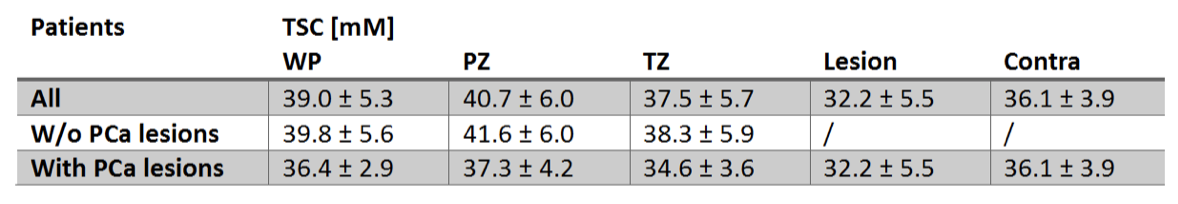
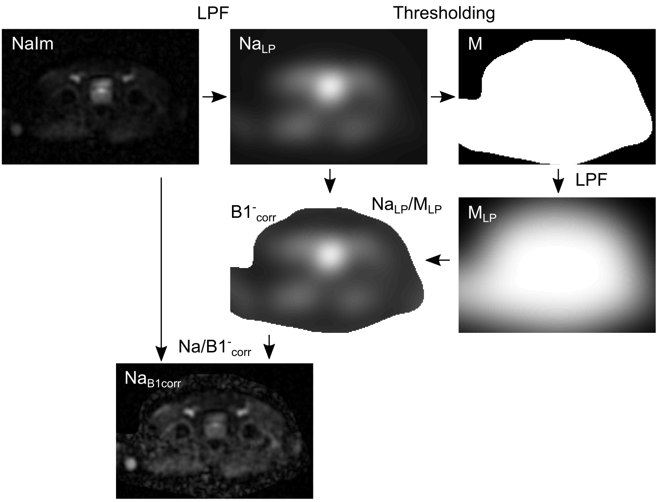
Figure 1: Illustration of the workflow correcting for B1- inhomogeneities in the 23Na MRI by application of two low pass filters (LPF). The algorithm was adapted from Lachner et al. (16).
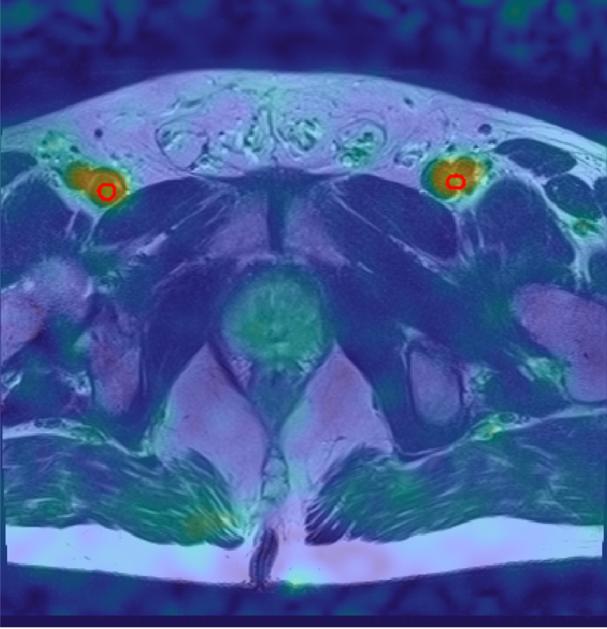
Figure 2: Transverse slice of one 23Na MR image with the segmentation of FBV for TSC quantification (red). The 23Na MR image was co-registered to the 1H MR image acquired with T2w turbo-spin echo and is shown as an overlay.
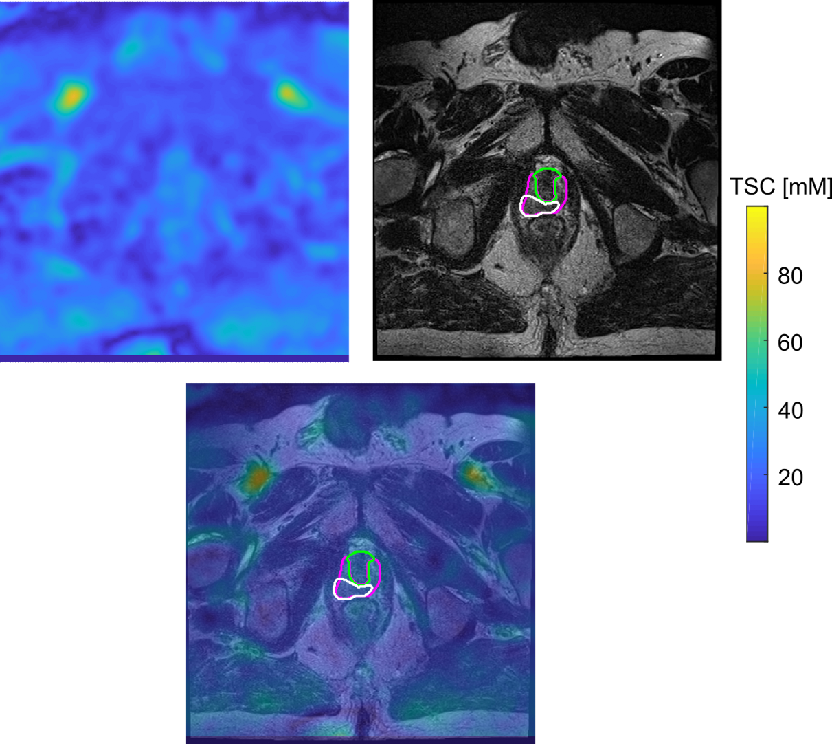
Figure 3: Transverse slice of the 23Na MR image (top left) and the 1H T2w TSE (top right) with segmentation of PZ, TZ, and one lesion within the TZ. Overlay of both images, including the segmented regions (bottom).