1831
Motion compensated multi-contrast MRI using deep factor model
Yan Chen1, James H. Holmes1, Curtis A. Corum2, Vincent Magnotta1, and Mathews Jacob1
1University of Iowa, Iowa City, IA, United States, 2Champaign Imaging, LLC, Minneapolis, MN, United States
1University of Iowa, Iowa City, IA, United States, 2Champaign Imaging, LLC, Minneapolis, MN, United States
Synopsis
Keywords: Motion Correction, Multi-Contrast
Recent quantitative parameter mapping methods including MR fingerprinting collect a time series of images that capture the evolution of magnetization. The focus of this work is to introduce a novel approach termed as deep factor model, which offers an efficient representation of the multi-contrast image time series. The higher efficiency of the representation enables the acquisition of the images in a highly undersampled fashion, which translates to reduced scan time in 3D high-resolution multi-contrast applications. The approach integrates motion estimation and compensation, making the approach robust to subject motion during the scan.Background
MR fingerprinting (MRF)1 and multi-contrast methods including MPnRage2 are emerging as time-efficient alternatives for classical MR sequences. They acquire an image time series in a highly undersampled fashion during magnetization evolution, followed by pixel-by-pixel fitting to derive the parameter maps. The images are often recovered using gridding or low-rank methods3-5. The estimated images' quality hinges on the multi-contrast images' quality; a more efficient joint recovery algorithm will translate to improved images and/or faster acquisition. A challenge with the above strategy is the subject motion during the scan that impacts joint reconstruction algorithms and pixel-by-pixel parameter fitting6,7.Deep Factor Model (DFM)
We introduce a deep factor model (DFM), which generalizes low-rank methods, for the representation and recovery of multi-contrast MRI data. The data is acquired using a 3D radial sequence with intermittent inversion pulses (see Fig.1). We assume the magnetization evolution during each inversion block to be identical. Ignoring transients and motion, we model the measurement at the time instant $$$t$$$ as $$ \mathbf y_t = \mathbf A_t \left(\boldsymbol\rho_{\tau(t)}\right) + \mathbf n_t,$$ where $$$\tau$$$ is the delay from the previous inversion pulse.DFM models each image using a conditional convolutional network (CNN) as (see Fig. 2) $$\boldsymbol\rho\left(\mathbf r,\tau\right)= \mathcal N_{ \theta, \phi}(\boldsymbol \gamma,\tau).$$ The input to the network $$$\boldsymbol \gamma$$$ is obtained by binning the k-t space data to eight bins based on $$$\tau$$$, followed by gridding. The DFM architecture derives the temporal factors $$$v(\tau)$$$, which modulate the features of $$$ \mathcal U$$$, using a fully-connected network $$$\mathbf v(\tau) = \mathcal V_{\boldsymbol \theta}(\tau)$$$8. The image is obtained as $$$ \boldsymbol\rho(\mathbf r,\tau) = \mathcal U_{\boldsymbol \phi}\left(\boldsymbol \gamma(\mathbf r),\mathbf v(\tau)\right)$$$.
We determine $$$\theta$$$ and $$$\phi$$$ by minimizing the loss: $$ \{\theta^*, \phi^*\} = \arg \min_{ \theta,\phi} \sum_t \left\|\mathbf y_t - \mathbf A_t\big(\mathcal N_{ \theta, \phi}(\gamma,\tau)\big)\right\|^2.$$ This unsupervised approach learns a patient specific network; it does not require any training data.
DFM with motion compensation (DFM-MC)
We model the subject motion at $$$t$$$ by $$$\nu$$$ and $$$\delta$$$, which are rotation and translation parameters. Using Fourier relations between rigid body motions and Fourier transform, we absorb these parameters to the forward model. These time-varying parameters are assumed to be unknowns and are solved during signal recovery as $$\{\theta^*,\phi^*, \{\nu_t, \delta_t\}\} = \arg \min_{\theta,\phi} \sum_t \|\mathbf y_t - \mathbf A_{t,\nu_t,\delta_t}\big(\mathcal N_{\boldsymbol \theta,\boldsymbol \phi}(\gamma,\tau)\big)\|^2.$$Results
The data was acquired from a normal volunteer on a GE 3T Premier scanner with 50K spokes with a tiny golden angle view ordering and a matrix size of 256$$$^3$$$ in 4.3 minutes. Inversion pulses were applied every 800 spokes, and a 500ms delay was applied for magnetization recovery to a steady state.We used a $$$\mathcal U_{\phi}$$$ network with three CNN layers, each with 16 features, while the $$$\mathcal V_{\theta}$$$ network used two dense layers, each with 16 features.
Validation of DFM in the absence of motion (Fig. 3): We compare DFM against the low-rank approach with two different ranks. We observe that the low-rank model offered a poor fit to the magnetization when rank=4, while rank=8 translated to noisy reconstructions. The DFM method can offer an improved tradeoff between accuracy and noisy artifacts resulting from undersampling. The plots of the voxel intensity profiles from gray matter(GM), white matter(WM), and cerebral spinal fluid(CSF) regions show that the DFM curves are closer to the expected magnetization during inversion recovery, which is similar to the rank=8 setting.
Validation of DFM-MC (Fig. 4): We acquired two datasets, one where the subject was instructed to hold still, and another where the subject was instructed to move multiple times during the scan. The results Fig. 4 (middle row) show that the proposed approach is able to compensate for the quite significant motion (bottom row) and offer reconstructions that are more comparable to the motion-free setting (top row). The estimated rotation and translation parameters are shown below.
Conclusion
We introduced a deep factor model (DFM) to represent and reconstruct multi-contrast MRI data in the context of inversion recovery radial acquisitions. The DFM used a conditional CNN model to represent each image in the time series as a non-linear function of the inversion delay time. Motion parameters were also treated as variables and solved in the DFM-MC formulation. The network and motion parameters were estimated from the data in an unsupervised fashion. The results show that the DFM model can offer improved tradeoffs over classical low-rank models. The DFM-MC approach is observed to compensate for motion in the multi-contrast data, and offer results that are comparable to a motion-free setting.Acknowledgements
This work is supported by NIH R01AG067078. This work was conducted on an MRI instrument funded by 1S10OD025025-01.References
- Ma D, Gulani V, Seiberlich N, et al. Magnetic resonance fingerprinting[J]. Nature, 2013, 495(7440): 187-192.
- Kecskemeti S, Samsonov A, Hurley S A, et al. MPnRAGE: A technique to simultaneously acquire hundreds of differently contrasted MPRAGE images with applications to quantitative T1 mapping[J]. Magnetic resonance in medicine, 2016, 75(3): 1040-1053.
- Mazor G, Weizman L, Tal A, et al. Low‐rank magnetic resonance fingerprinting[J]. Medical physics, 2018, 45(9): 4066-4084.MLA.
- Assländer J, Cloos M A, Knoll F, et al. Low rank alternating direction method of multipliers reconstruction for MR fingerprinting[J]. Magnetic resonance in medicine, 2018, 79(1): 83-96.
- Zhao B, Setsompop K, Adalsteinsson E, et al. Improved magnetic resonance fingerprinting reconstruction with low‐rank and subspace modeling[J]. Magnetic resonance in medicine, 2018, 79(2): 933-942.MLA.
- Kecskemeti S, Samsonov A, Velikina J, et al. Robust motion correction strategy for structural MRI in unsedated children demonstrated with three-dimensional radial MPnRAGE[J]. Radiology, 2018, 289(2): 509.
- Lee H, Zhao X, Song H K, et al. Self-navigated three-dimensional ultrashort echo time technique for motion-corrected skull MRI[J]. IEEE transactions on medical imaging, 2020, 39(9): 2869-2880.
- Huang X, Belongie S. Arbitrary style transfer in real-time with adaptive instance normalization[C]//Proceedings of the IEEE international conference on computer vision. 2017: 1501-1510.
Figures
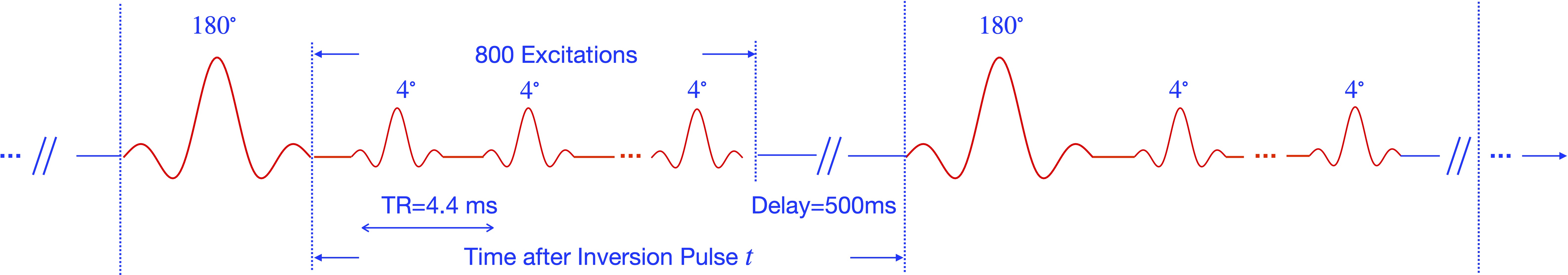
Fig. 1. Illustration of the pulse sequence. The data were acquired using an inversion recovery sequence with a segmented readout consisting of a train of ultrashort echo-time 3D radial acquisitions with TR=4.4ms. Intermittent adiabatic inversion pulses were applied after 800 UTE radial lines, with a delay of 500 ms after each acquisition block to allow for signal recovery to a steady state. The total acquisition time was 4.3 minutes to acquire 50K spokes with a matrix of 256$$$^3$$$. We used the tiny golden angle view order. The field of view (FOV) was 24cm$$$^3$$$
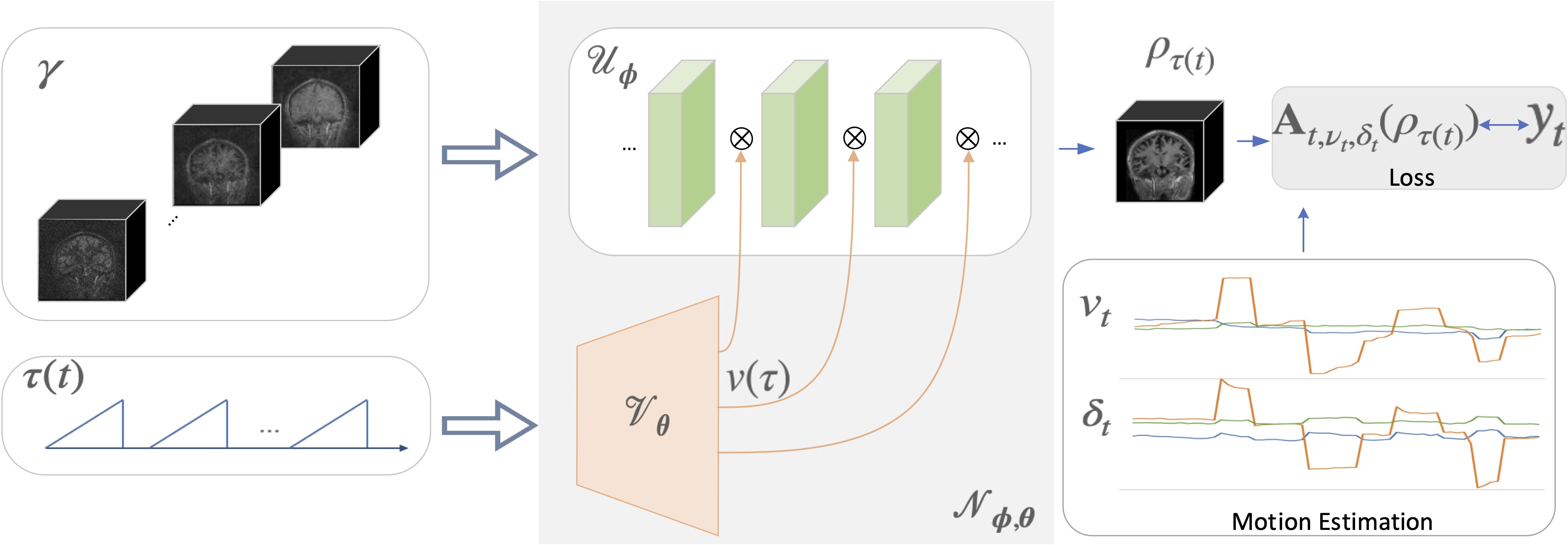
Fig. 2. Illustration of DFM, which represents the signal $$$\rho(\mathbf r,\tau)$$$ as the output of a conditional network $$$\mathcal N_{\phi,\theta}$$$. The features of the CNN $$$\mathcal U_{\phi}$$$ are modulated by $$$v(\tau)$$$, that are generated by a fully-connected network $$$\mathcal V_{\theta}$$$. The input to $$$\mathcal V_{\theta}$$$ is $$$\tau$$$, while that of the $$$\mathcal U_{\phi}$$$ is an approximate initialization $$$\boldsymbol{\gamma}$$$. These volumes are obtained by grouping the radial lines based on $$$\tau$$$ and gridding.
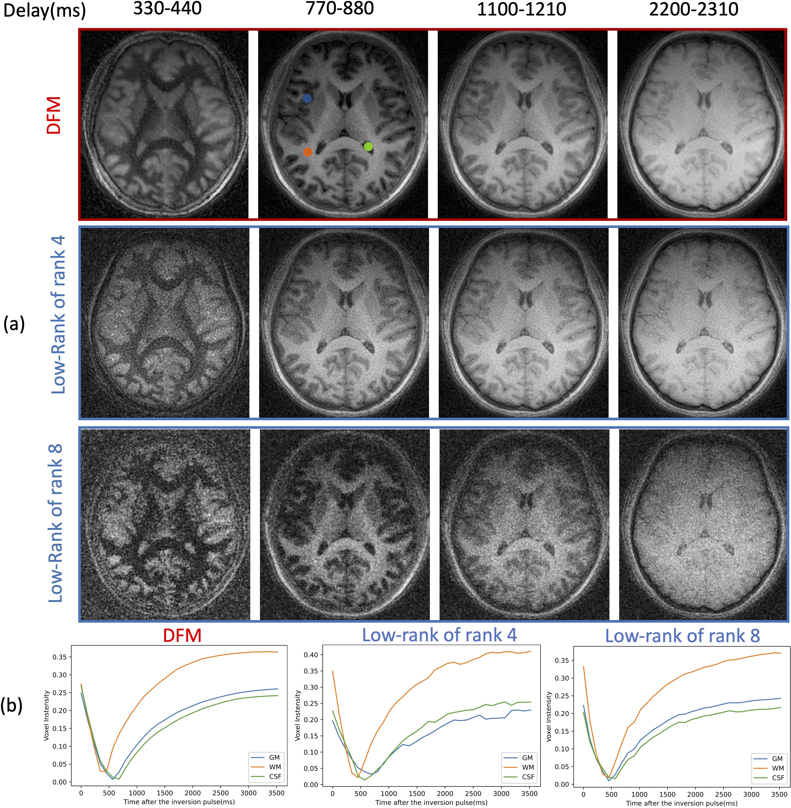
Fig. 3. Validation of DFM in the absence of motion. The data was reconstructed with DFM and low-rank methods with two ranks. (a) The four columns correspond to four delay times $$$\tau$$$ after one inversion pulse; (b) Magnetization recovery curve of gray matter(GM), white matter(WM), and cerebral spinal fluid (CSF) voxels (whose locations are indicated by the colored dots in the top image), estimated by different approaches. The experiments show that DFM offers an improved tradeoff between the suppression of noisy alias artifacts and the accuracy of magnetization recovery curves.
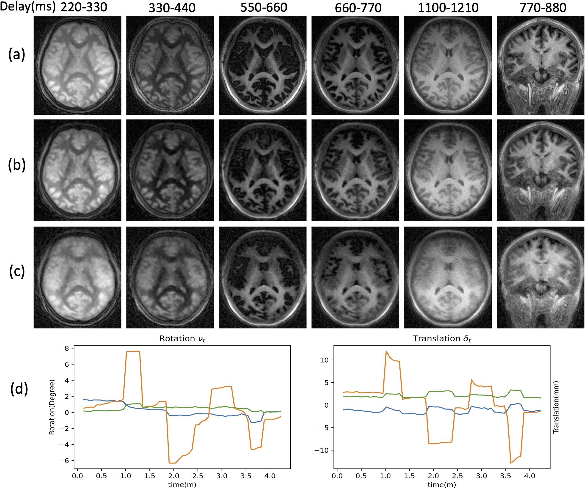
Fig. 4. Validation of DFM-MC. The first five columns correspond to an axial view with different delays, while the last corresponds to a coronal view. (a) DFM reconstruction of the dataset without motion; (c) DFM reconstruction of the dataset with motion (b) DFM-MC reconstruction of the dataset with motion (d) Estimated motion parameters including rotation and translation to correct (c) to (b). The results show that DFM-MC can compensate for motion effects and offer reconstructions that are more comparable to DFM reconstructions of the dataset without motion.
DOI: https://doi.org/10.58530/2023/1831