1804
Joint fitting of ADC and R2 with an estimate of the signal offset improves noise characteristics of whole-body R2 maps.1The Institute of Cancer Research, London, United Kingdom, 2The Royal Marsden NHS Foundation Trust, London, United Kingdom
Synopsis
Keywords: Quantitative Imaging, Modelling
Joint fitting of ADC and R2 improves the noise characteristics of whole-body R2 maps when using an iterative weighted least squares (IWLS) estimation that accounts for the signal offset, ρ, between diffusion-weighted and multi-echo-time imaging sequences. This is demonstrated using simulation experiments using relevant values of R2, ADC, and signal-to-noise ratio (SNR), where we find an improvement in R2 precision using the joint-fitting approach. Initial validation was further performed in clinical imaging examples to demonstrate the improvement in R2 map detail.Introduction
The utility of the apparent diffusion coefficient (ADC) and R2 has been examined in many clinical applications[1–6]. Although previous studies have investigated joint fitting of ADC and R2 using identical EPI protocols in pulmonary disease[7], to our knowledge no studies have investigated whole-body estimation for evaluation of metastatic disease. Furthermore, previous attempts at joint fitting of ADC and R2 do not account for differences in signal intensities between DWI and multi-echo-time sequences acquired as separate acquisitions.In this study we (i) propose an updated signal model for joint ADC/R2 fitting, (ii) compare iterative weighted least-squares (IWLS) versus ordinary least-squares (OLS) for joint ADC/R2 fitting using simulation experiments, and (iii) demonstrate the utility of whole-body ADC/R2 estimation in a patient with metastatic melanoma.
Methods
i) Updated signal model for joint ADC/R2 fittingImplementing joint ADC/R2 fitting on a clinical MRI scanner may require acquisition of the sequences for the estimation of R2 (multi-TE data) and DWI data separately. Variation in receiver gain between separate acquisitions will affect signal intensity, which impairs joint fitting. We model this offset by the variable factor ρ such that the models for DWI and multi-TE data become:
$$\begin{gathered}S_{\mathrm{DWI}}\left(b_i,\mathrm{TE}_{\mathrm{DWI}}\right)=\rho S_0\exp\left(-b_i * \mathrm{ADC}\right)\exp\left(-\mathrm{TE}_{\mathrm{DWI}}*\mathrm{R}_2\right)+\varepsilon_i \\S_{\mathrm{R}_2}\left(\mathrm{TE}_i\right)=S_0\exp\left(-\mathrm{TE}_i*\mathrm{R}_2\right)+\varepsilon_i\end{gathered}$$ (Equation 1).
$$$\varepsilon_i$$$ is assumed to be zero-mean Gaussian-distributed noise with standard deviation, σ.
ii) Comparing OLS and IWLS
Following linearisation of data using log-transformation of Equation 1, OLS fitting can estimate the values of ρ, S0, ADC and R2 for known values of $$$b_i$$$, $$$\mathrm{TE}_{\mathrm{DWI}}$$$ and $$$\mathrm{TE}_i$$$. A drawback is that it incorrectly assumes homoscedastic noise variance in the data after log-transformation, which is known to be false. IWLS optimisation can improve this for ADC fitting[8] and so we compared OLS and IWLS strategies.
To match our clinical protocol, DWI data were generated according to Equation 1 using b-values of 50, 600, and 900 s/mm2 (repeated 12 times) with $$$\mathrm{TE}_{\mathrm{DWI}}$$$=73 ms; multi-echo-time data were generated with TE=39/118 ms (repeated twice); ADCtrue=1.5x10⁻³mm2/s and R2true=0.02 s-1. S0=1 and Rician-distributed noise was added to the generated data with variance=1/SNR2 where SNR={5,10,20,50,100,200,300} and $$$\rho\in(0,0.25, \ldots,2)$$$ for each value of SNR. ADC and R2 were estimated using IWLS and OLS using three approaches: (a) separate fitting of DWI and multi-TE data, (b) joint-fitting, including estimation of ρ, and (c) joint fitting assuming ρ=1. The bias in the estimate of parameter X was defined as:
$$\operatorname{bias}(\widehat{\mathrm{X}})=\frac{1}{N}\sum_{j=1}^N\frac{\widehat{\mathrm{X}}_j-\mathrm{X}^{\text{true}}}{\mathrm{X}^{\text{true}}}$$
and the variance was:
$$\operatorname{var}(\widehat{\mathrm{X}})=\frac{1}{N}\sum_{j=1}^N\frac{\left(\widehat{\mathrm{X}}_j-\mathrm{X}^{\text{true}}\right)^2}{\mathrm{X}^{\text{true}}}$$
for N=1000 simulation samples, where $$$\widehat{\mathrm{X}}$$$ is the estimated parameter.
iii) Whole-body ADC/R2 estimation
Data were acquired in a single patient with metastatic melanoma according to the protocol defined in the simulation study, with DWI acquired using EPI with bipolar diffusion-encoding gradients and using the same sequence with b=0 and monopolar diffusion-encoding at matched slice locations and resolution. Joint fitting with the IWLS algorithm was used to estimate a map of ρest which was smoothed to ρG using a gaussian filter (Figure 1). Maps of the ADC and R2 were recalculated using IWLS following rescaling of the DWI data using ρG.
Results
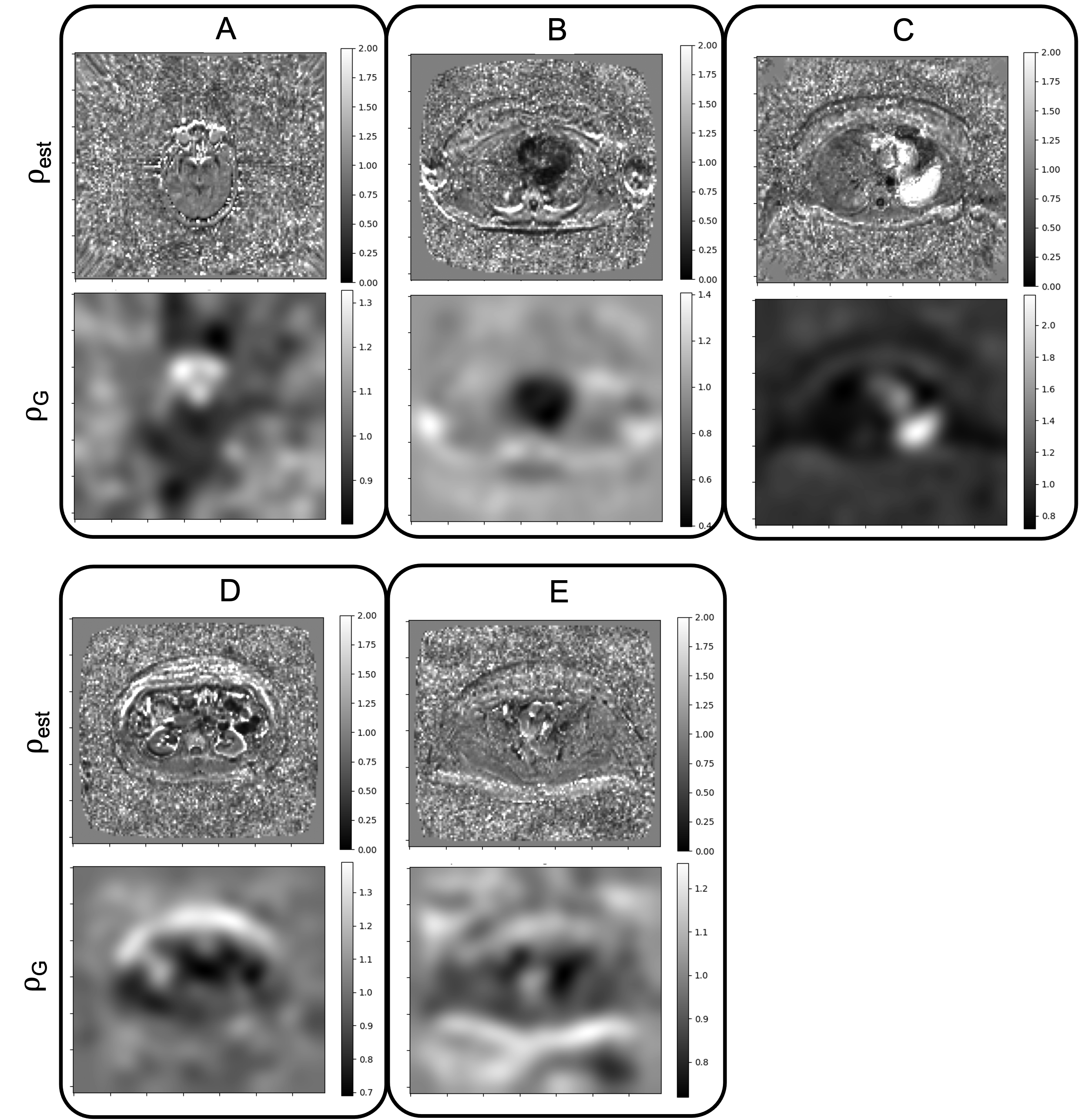
Figure 2 shows the changes in bias and variance of $$$\widehat{\mathrm{ADC}}$$$ and $$$\widehat{\mathrm{R_2}}$$$. For SNR>50, var($$$\widehat{\mathrm{ADC}}$$$) and var($$$\widehat{\mathrm{R_2}}$$$) are both reduced using IWLS (values for high SNR simulations shown in Figure 3). However, when ρ is assumed to be 1, bias is observed in estimation of these parameters.Figures 4 shows maps of ADC and R2, estimated separately or jointly using IWLS and smoothed ρG (Figure 5). In a single square ROI of 16 pixels drawn in healthy liver the variance of the pixel values was 2.6x10⁻⁵s-1 in the separately fitted R2 map and 9.0x10⁻⁶s-1 in the map estimated using IWLS and ρG.
Discussion
The separate fittings to the equations in Equation 1 show the same changes in the bias and variance for $$$\widehat{\mathrm{ADC}}$$$ and $$$\widehat{\mathrm{R_2}}$$$ as the joint fitting estimating ρest. When ρest=1, for ρ<1 bias($$$\widehat{\mathrm{ADC}}$$$) is reduced when using the IWLS method, however bias($$$\widehat{\mathrm{R_2}}$$$) is larger than with OLS for the same values. When ρest=ρ=1 and SNR>20 bias($$$\widehat{\mathrm{ADC}}$$$) and bias($$$\widehat{\mathrm{R_2}}$$$) are the same with both IWLS and OLS. Var($$$\widehat{\mathrm{ADC}}$$$) and var($$$\widehat{\mathrm{R_2}}$$$) are both reduced with IWLS for SNR>50 because the fitting has fewer degrees of freedom: the value of ρ is known.In the clinical case, values of ρest are shown to vary spatially across the image. Areas of flow, motion, small structures, or other mechanisms leading to localised signal loss result in overestimations of the ADC or R2 and extreme values of ρest. Smoothing to ρG magnifies this effect resulting in large differences in the ADC or R2 as seen in the spinal CSF and the aorta respectively. Further work is necessary to investigate the impact of smoothing ρest on the ADC and R2 maps.
While a significant change in the noise characteristics is not observed in the ADC map corrected with ρG, the corrected R2 map displays better signal homogeneity in central regions of the liver, spleen, and muscle.
Conclusion
Joint fitting of DWI and multi-TE data improves noise characteristics of the R2 map when using IWLS with a smoothed estimate of the signal gain factor, ρG. Further validation is necessary using quantitative measurements of the SNR and estimation of ρ using phantom and clinical experiments.Acknowledgements
This work represents independent research funded by the National Institute for Health and Care Research (NIHR) Biomedical Research Centre and the Clinical Research Facility in Imaging at The Royal Marsden NHS Foundation Trust and the Institute of Cancer Research, London. The views expressed are those of the authors and not necessarily those of the NIHR or the Department of Health and Social Care.References
1. Chen L, Liu M, Bao J, et al (2013) The Correlation between Apparent Diffusion Coefficient and Tumor Cellularity in Patients: A Meta-Analysis. PLoS One 8:e79008.
2. Koinuma M, Ohashi I, Hanafusa K, Shibuya H (2005) Apparent diffusion coefficient measurements with diffusion-weighted magnetic resonance imaging for evaluation of hepatic fibrosis. J Magn Reson Imaging 22:80–85.
3. Gass A, Niendorf T, Hirsch JG (2001) Acute and chronic changes of the apparent diffusion coefficient in neurological disorders—biophysical mechanisms and possible underlying histopathology. J Neurol Sci 186:S15–S23.
4. Wood JC, Enriquez C, Ghugre N, et al (2005) MRI R2 and R2* mapping accurately estimates hepatic iron concentration in transfusion-dependent thalassemia and sickle cell disease patients. Blood 106:1460.
5. Mai J, Abubrig M, Lehmann T, et al (2019) T2 Mapping in Prostate Cancer. Invest Radiol 54:146–152.
6. Thavendiranathan P, Walls M, Giri S, et al (2012) Improved Detection of Myocardial Involvement in Acute Inflammatory Cardiomyopathies Using T2 Mapping. Circ Cardiovasc Imaging 5:102–110.
7. Cheng L, Blackledge MD, Collins DJ, et al (2016) T2-adjusted computed diffusion-weighted imaging: A novel method to enhance tumour visualisation. Comput Biol Med 79:92–98.
8. Blackledge MD, Tunariu N, Zugni F, et al (2020) Noise-Corrected, Exponentially Weighted, Diffusion-Weighted MRI (niceDWI) Improves Image Signal Uniformity in Whole-Body Imaging of Metastatic Prostate Cancer. Front Oncol 10:704.
Figures
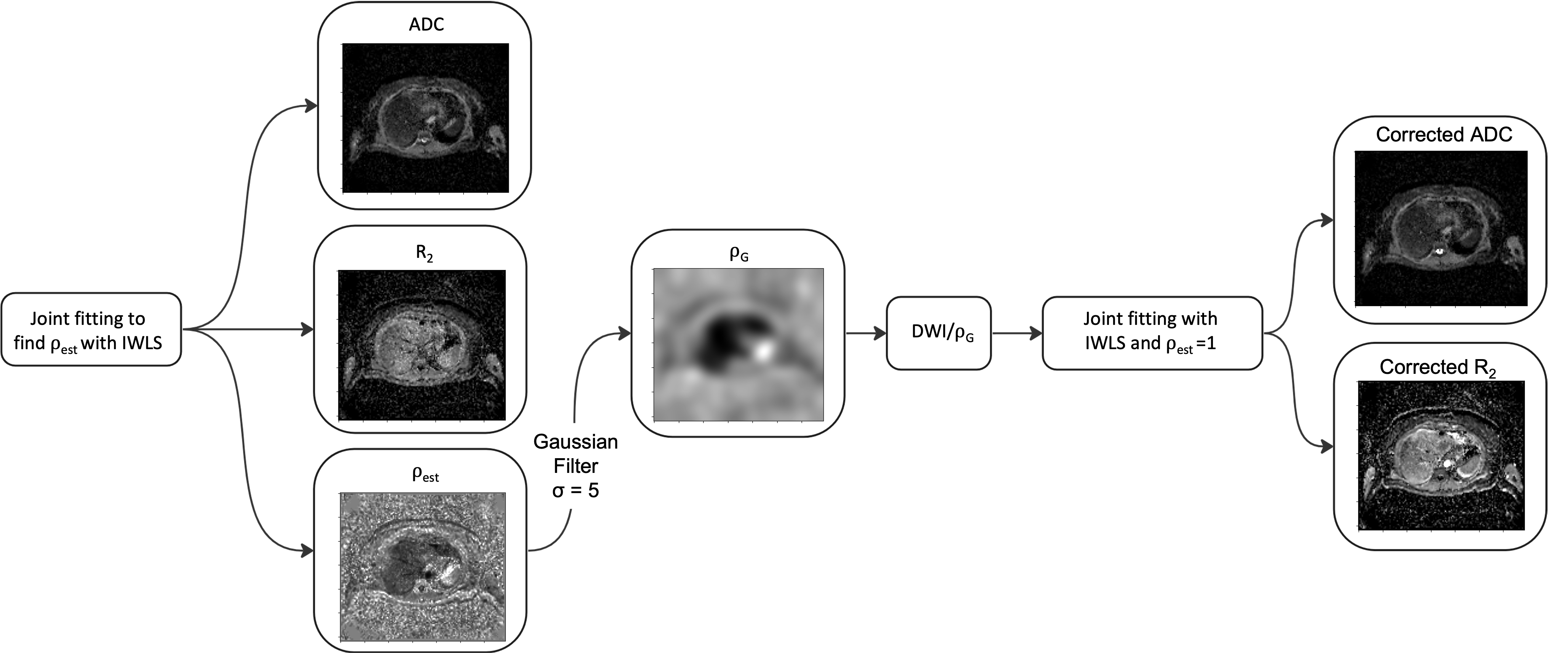
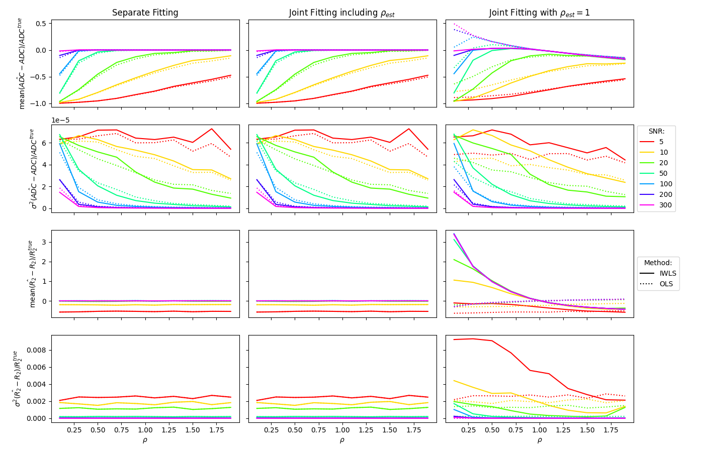
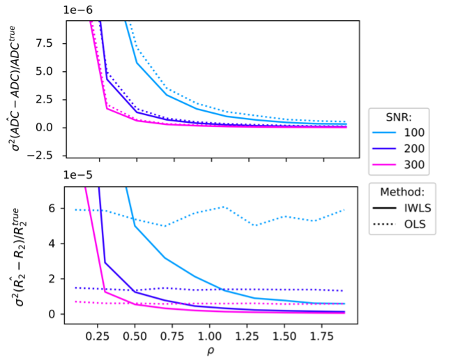

Figure 4: Five slices (A-E) from a single patient showing maps of the ADC and R2 plotted using a joint fitting estimating the ADC, R2, ρ and the signal when the echo time (TE) = 0 and b-value = 0 (S0), and corrected maps of the ADC and R2 after the DWI signal was divided by the corresponding value of ρG in Figure 5. There is a notable increase in the SNR of the R2 map. The windowing of images at each slice are matched.