Synopsis

Keywords: Low-Field MRI, Gradients

Open magnet provide advantageous facility for imaging the human body in a natural way. However field inhomogeneities can reduce the utilisable imaging field-of-view. We present a simple way to map the static field inhomogeneity and the non-linear gradient inhomogeneity in order to correct them during the image reconstruction.

Introduction

Open MRI scanners provide opportunities to study human physiology in a more natural way than in standard cylindrical-bore systems. However, the static field produced by an open magnet is more inhomogeneous than that of a cylindrical magnet, leading to image distortions and even some loss in signal. Furthermore, open scanners must use bi-planar gradient coils for spatial encoding, which generally provide reduced performance in terms of achievable gradient amplitude, switching rate and linearity. Interaction with the proximal iron pole pieces of the magnet can also produce spatiotemporal distortion of gradient waveforms. These result in spatial and potentially, temporal inhomogeneities of the magnetic fields, causing deviations from the desired k-space trajectory during imaging. The resulting performance is sufficient for slow imaging of static objects, but hampers rapid imaging of dynamic processes, for which the upright geometry is particularly valuable. Hardware and reconstruction development makes it possible to monitor the magnetic field using field probes¹, as well as using image specific phantoms^2,3. The correct k-space trajectory can thus be used to correct the sampled acquisition for reconstruction based on the subject position regarding the gradient fields at the time of the acquisition^4,5. We propose to evaluate the magnetic field affected by temporal gradient non-linearity (GNL) within a typical field of view (FOV) required for body imaging using a purposed-made phantom with a known ground truth. Using a reversed-gradient sequence and a non-linear registration algorithm, we estimated the static magnetic field and gradient distortion in an open scanner.

Methods

Data were acquired on a 0.5T ASG-Paramed MROpen scanner, using a 4-channel receiver spinal coil. A tray made of two sheets of Plexiglas with laser-cut holes equally sampled every 25mm was fixed on the bed of the MRI scanner. A total of 104 spheres of 10mm diameter were filled with pure water and arranged on the tray to cover a surface of 250x250mm². A few positions were left empty to allow pattern recognition. The imaging sequence was a 3D Gradient echo sequence (TE/TR=5/12.4ms, FA=10^o, FOV=500x500x100mm and isotropic voxels of 2.5mm³,total of 40 slices), with a bandwidth readout=27.5kHz (scan time=5min per direction). The planning was specified to have the centre of the FOV at the magnet/gradient isocentre, with the possibility to reverse the readout gradient direction. Images with the readout gradient in the +z and -z directions were acquired and retrospectively registered using the non-linear registration algorithm fnirt⁶ to obtain a map of the static field inhomogeneities. Subsequently the corrected image was registered using fnirt to a ground truth image based on the known phantom geometry created using ITK-snap⁷. The obtained field warp was then fitted at the centre of each sphere using a 3^rd degree polynomial surface before being extrapolated to the whole FOV using matlab. The resulting map was then scaled to show the measured ball position in mm in each Cartesian direction. In a separate experiment, 4 field probes⁸ were used to monitor the time-course of the z-gradient in a pulse-acquire sequence where the gradient pulse of interest G_z was shifted through the acquisition window. The duration of the gradient was 5ms with a rise time of 0.6ms for an amplitude of 4mT/m (20% of maximum gradient strength) and the acquisition window was 11ms (TR=50ms), for a total number of acquisitions of 12890 (Number of signal averages = 10). The derivative of the phase of the FID signal was computed to extract the frequency, and therefore the magnetic field strength at a point. A pointwise moving overlap averaging was used and the profile subsequently filtered with a cut-off of 6 kHz. The field probes were positioned at 0mm, +60mm, +120mm and -120mm from the isocentre of the magnet in the z-direction.

Results

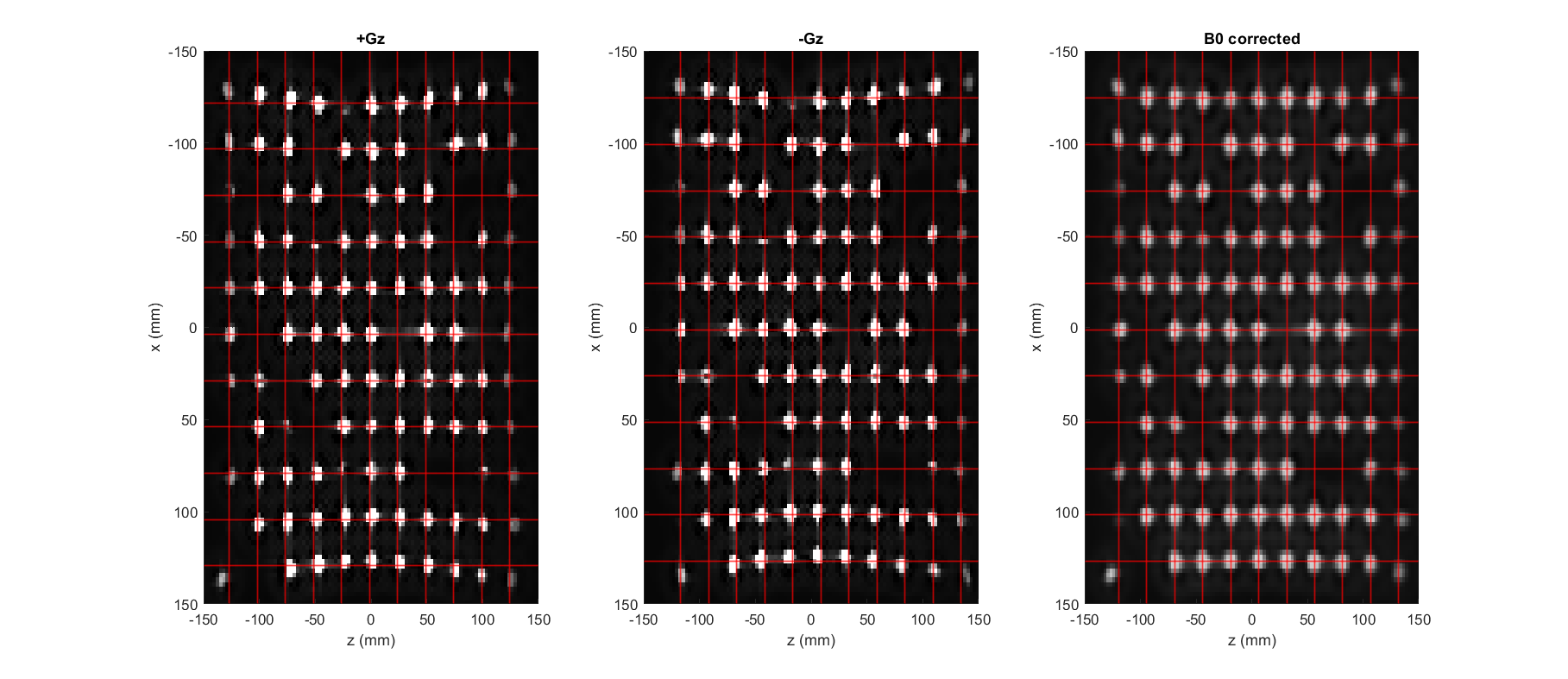
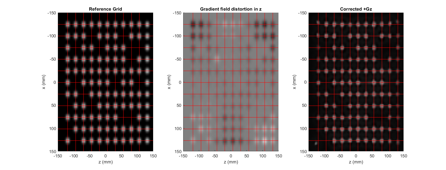
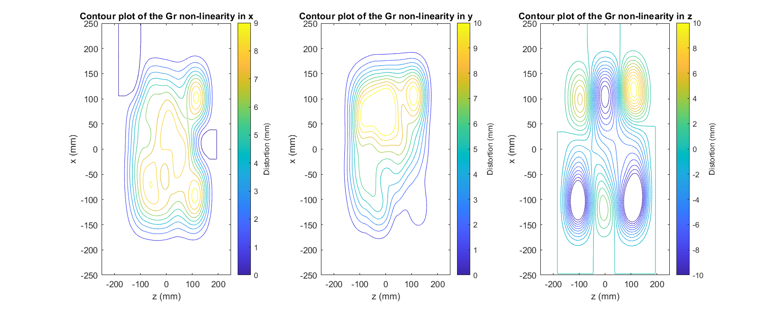
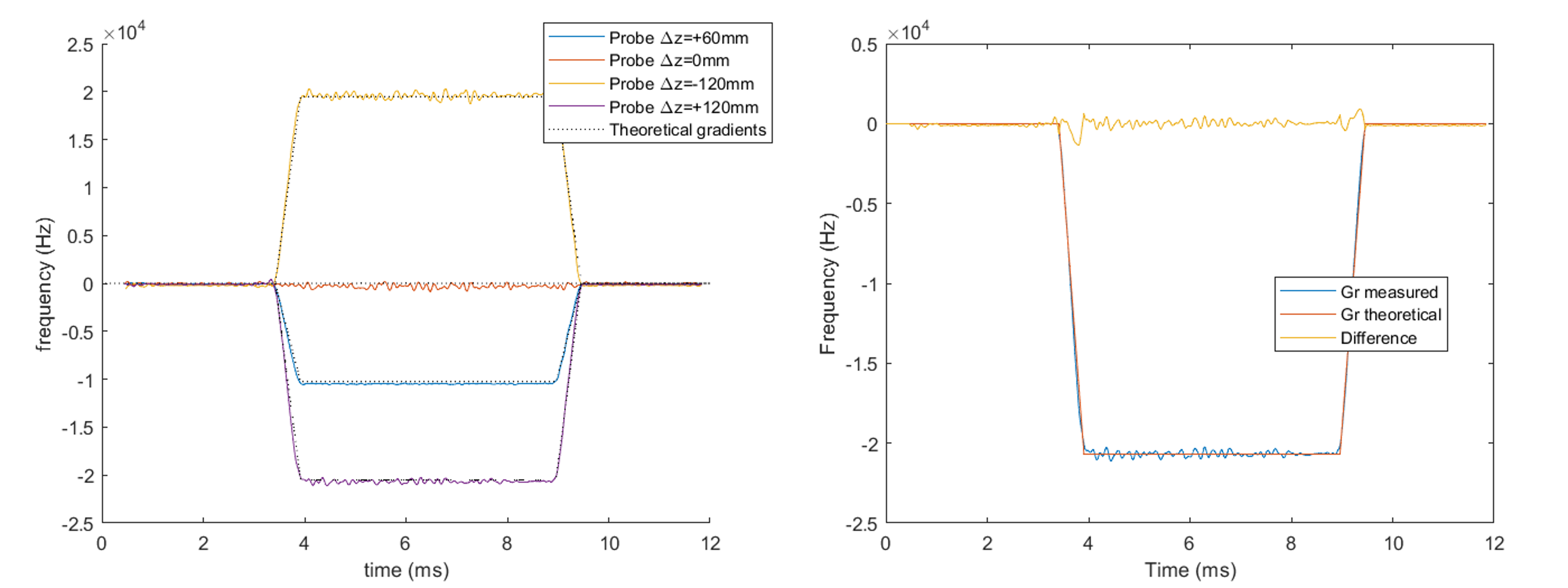
The gradient reversal in the z direction allowed effective correction of the distortion due to static field inhomogeneities, as shown in the Figure 1. From a generated image of spheres on the reference grid (Figure 2a), it was possible to estimate the resulting gradient distortions in the three Cartesian directions, as shown with the contour plots of the Figure 3. The temporal characteristics of the gradients were measured using fields probes and show good SNR with the expected polygon shape requested in the sequence, as shown in figure 4.

Discussion

A non-linear registration algorithm was used to estimate the displacement of the various spheres both due to static magnetic field inhomogeneity and gradient non-linearity. The registration could be improved to provide better precision in the estimated displacement, but it would have little influence on the resulting low-varying gradient variation that could be observed on the figure 3. However, it was still possible to record distortion of up to ±10mm in a FOV=500mm. The gradient waveforms conformed well to the expected waveforms and showed no detectable change in shape across the FOV. The measured maps and gradient waveforms will be incorporated into a model-based reconstruction and solved iteratively as described in⁴ to improve the spatial resolution and FOV coverage at 0.5T.

Conclusion

Gradient non-linearity was mapped successfully using a grid-like phantom and image registration algorithm after correcting for the effects of the B₀ inhomogeneity using a gradient reversal sequence on a 0.5T Upright Open scanner.

Acknowledgements

This research was supported but the EPSRC Grant EP/V025856/1.