1764

Denoising Simulated Low-Field MRI (70mT) using Denoising AutoEncoders (DAE) and Cycle-Consistent Generative Adversarial Network (Cycle-GAN)

Fernando Vega^1,2,3, Abdoljalil Addeh^1,2,3, and M. Ethan MacDonald^1,2,3,4
¹Biomedical Engineering, University of Calgary, Calgary, AB, Canada, ²Electrical & Software Engineering, University of Calgary, Calgary, AB, Canada, ³Hotchkiss Brain Institute, University of Calgary, Calgary, AB, Canada, ⁴Department of Radiology, University of Calgary, Calgary, AB, Canada

Synopsis

Keywords: Low-Field MRI, Machine Learning/Artificial Intelligence, MRI, Unpaired Image Translation

In this work, a denoising Cycle-GAN is implemented to yield high-field, high resolution, high signal-to-noise ratio MRI images from simulated low-field, low resolution, low signal-to-noise MRI images. Resampling and additive Rician noise were used to simulate low-field MRI. Images were utilized to train a DAE and Cycle-GAN, with paired and unpaired cases, respectively. Both networks were evaluated using SSIM and PSNR image quality metrics. This work demonstrates the use of advanced machine learning to improve low-field MRI images that can outperform classical denoising autoencoders and does not require image pairs.

Introduction

Over the last few decades there has been an increasing use of magnetic resonance imaging (MRI) as it provides hundreds of contrast modes and is minimally invasive.^1,2 It is known that higher spatial resolution and SNR-efficiency can be achieved with higher field strength³, however, as the field strength increases so does the cost.⁴ Low-Field MRI scanners are less expensive (~20× less expensive than 3T over 10 years), have much lower energy consumption (~60× less electricity)⁵, reduced the energy absorption into the subject, and they do not require expensive liquid helium⁶; however, the trade-off of is lower resolution, and lower SNR-efficiency.⁷

Previous work aimed to improve the resolution and SNR-efficiency by implementing machine learning techniques such as a denoising autoencoder (DAE)^8,9 that uses Convolutional Neural Networks (CNN)¹⁰, however, using this architecture requires the images to be paired and aligned. Performing registration in noisy images is prone to error, therefore, we improved upon the previous work by replacing the DAE with a cycle-consistent generative adversarial network (Cycle-GAN)¹¹ that does not require the images to be paired or registered as a DAE does.

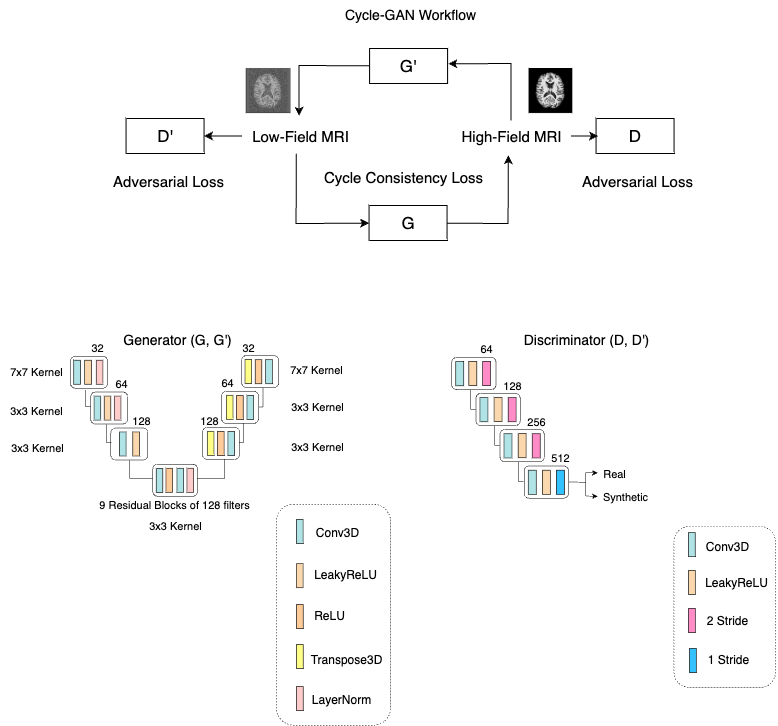
Cycle-GAN architecture is also based on CNNs, it uses four networks: two generator and two discriminators where one generator produces synthetic denoised images that is fed to second generator that generates the original the noisy image, one discriminator is assigned to each generator to estimate if the generated images are real or synthetic.¹² Using this approach GANs architectures excel on generating synthetic images with high degree of similarity to the real ones.¹³

In this work, a 3D Cycle-GAN was implemented using unpaired 3T MRI images and low-field simulated MRI images. The model was evaluated with unseen images and reported the Structural Similarity Index (SSIM)¹⁴ and Peak Signal-to-Noise Ratio (PSNR)¹⁵ as performance metrics. These results are compared with DAE performance

Methods

100 T1-weighted MRI images were used from Open Access Series of Imaging Studies (OASIS-3)¹⁶ database (3T MRI images with a resolution of 1mm×1mm×1mm). Then low-field MRI images were synthesised to have a resolution of 1.5mm×1.5mm×5mm and added Rician noise to emulate low SNR of 70mT.¹⁷

A 3D Cycle-GAN model was implemented using the MONAI deep learning framework¹⁸, the model was fed with 100 high-field MRI images and 100 simulated low-field MRI images for 500 epochs and follows the architecture shown in Figure 1. This architecture has a 15 total layers with 9 residual blocks that act as a bottleneck without any skip connection, as shown in Figure 1, this architecture diverges from the standard U-net style followed in DAE.

Once the model was trained, it was evaluated with 100 unseen images and compared with results from a DAE and evaluated with respect to the structural similarity index measure (SSIM) and peak signal-to-noise ratio (PSNR).

Results

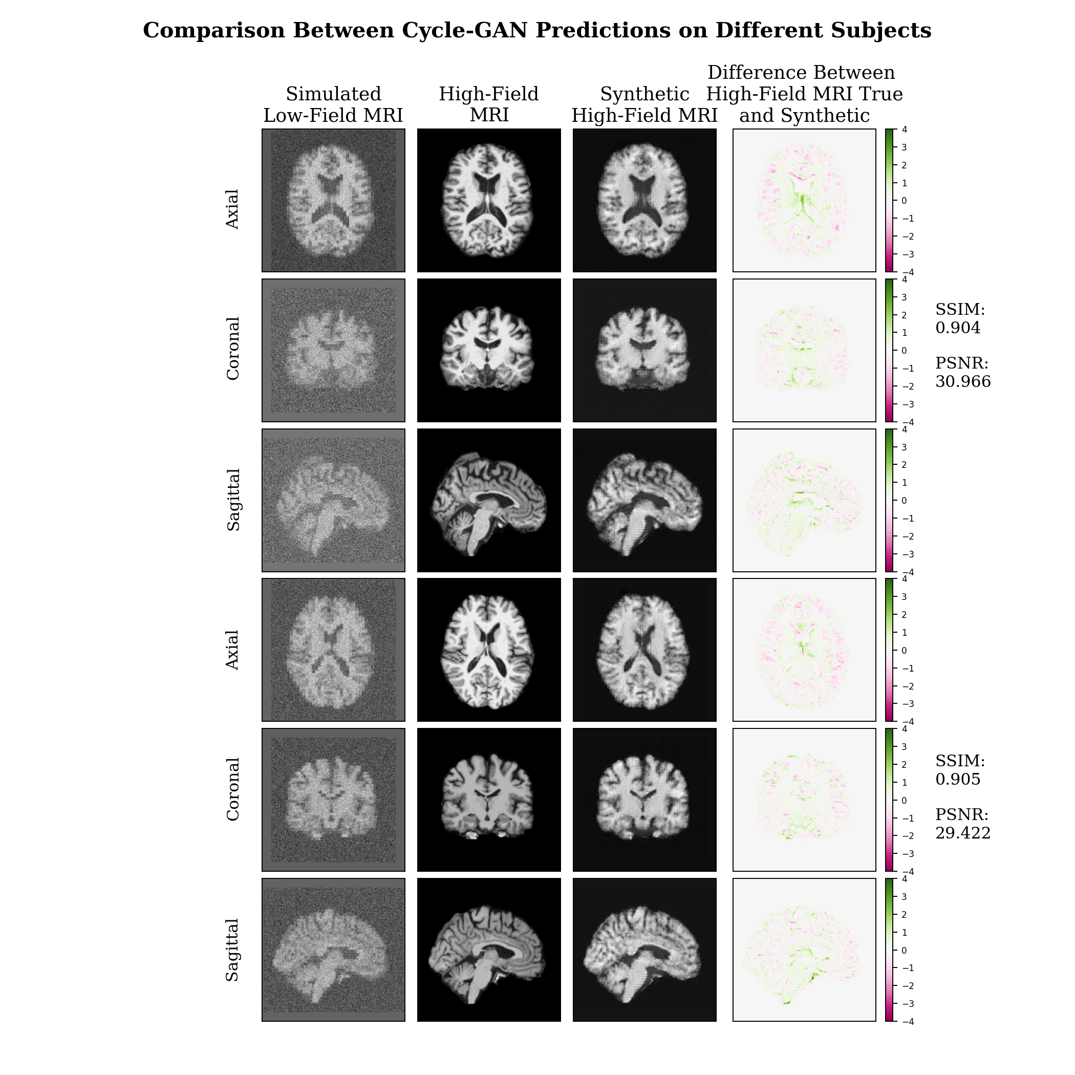
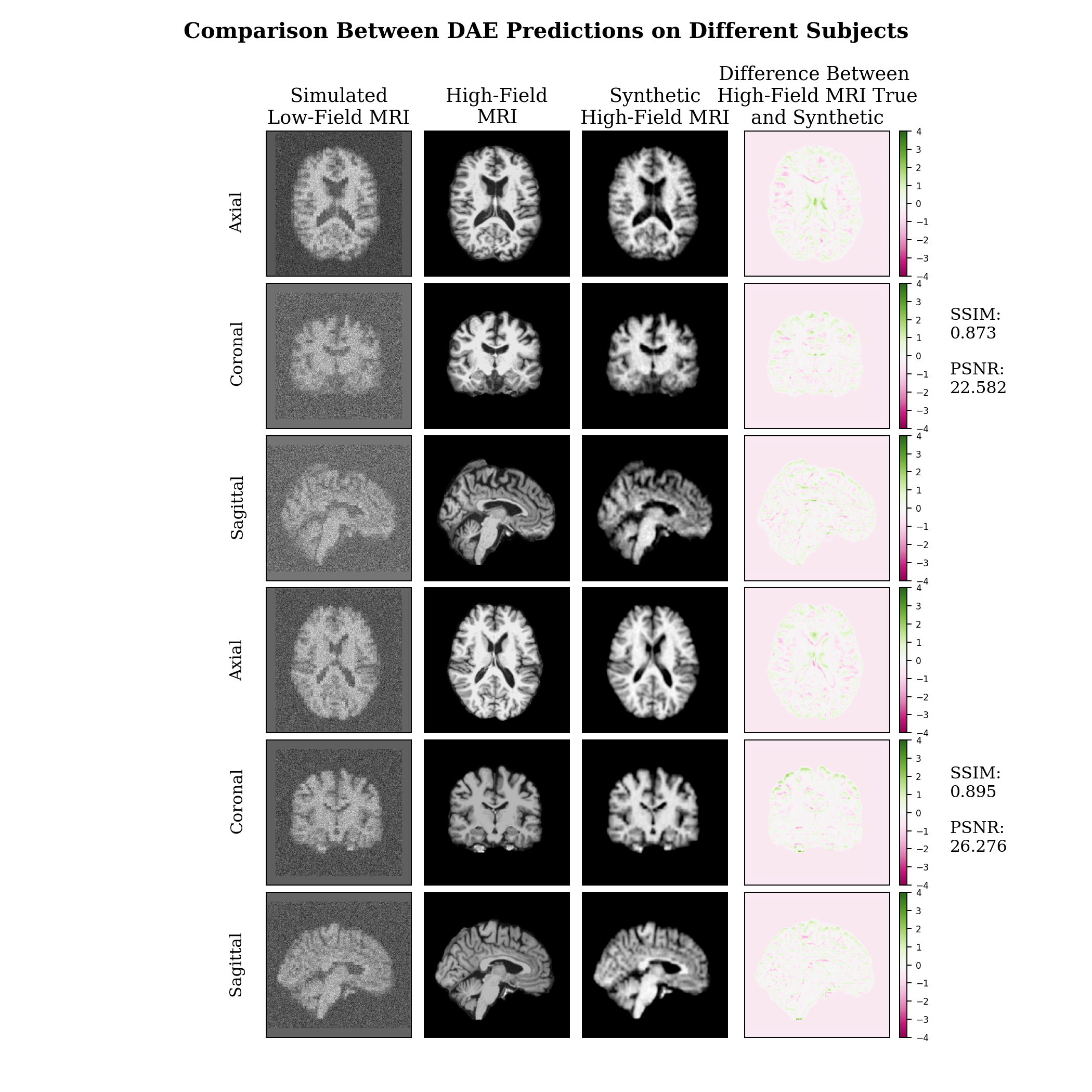
In Figure 2, the synthetic images have high degree of visual similarity with the true images and are quantitatively similar based on the SSIM and PSNR.

Figure 3 shows the same subjects using DAE.

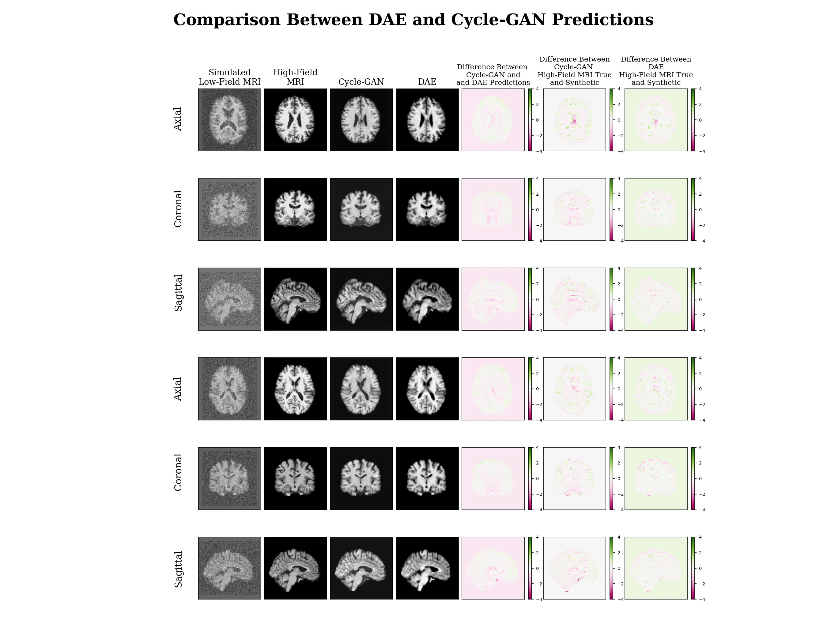
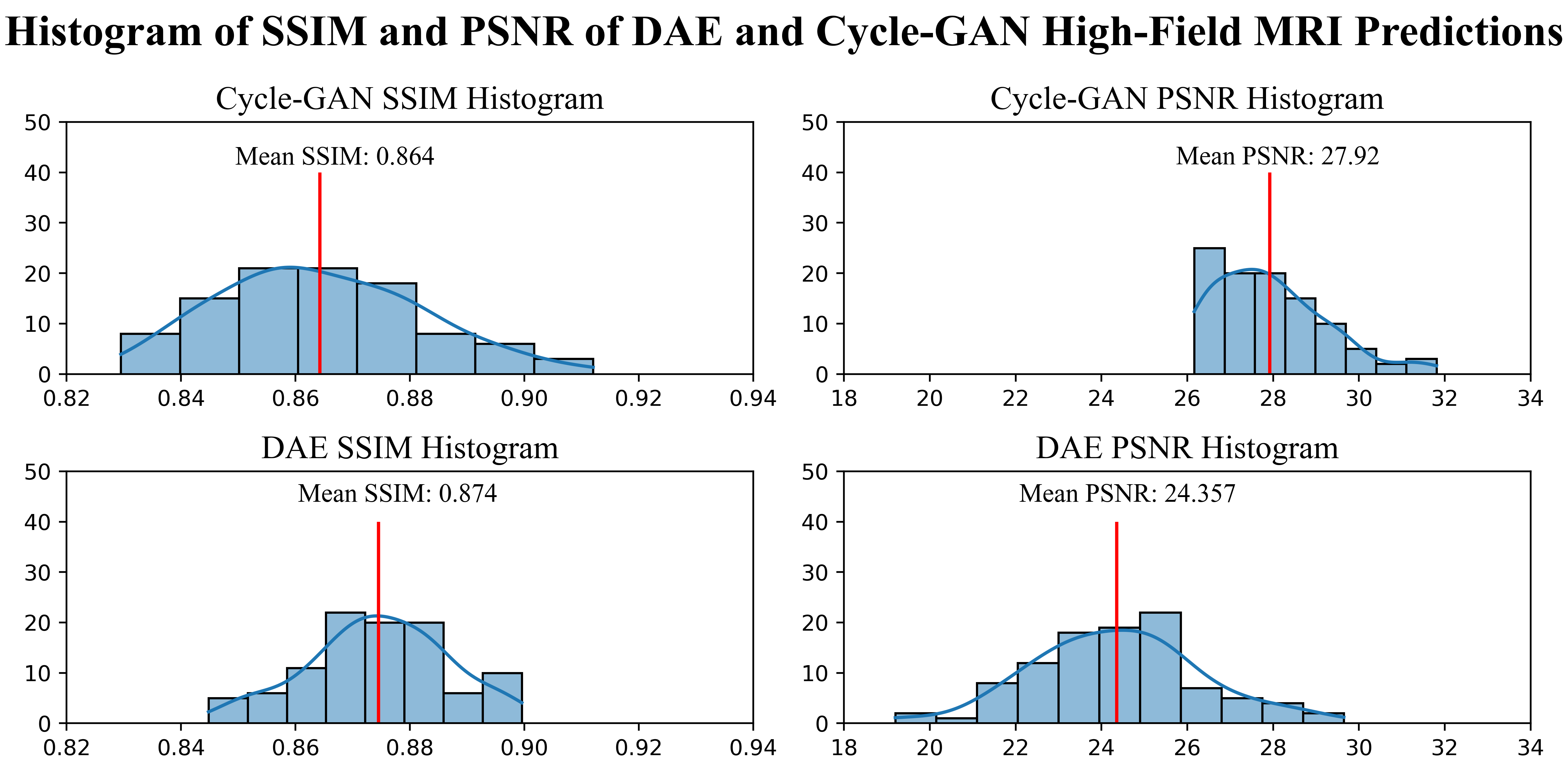
In Figure 4, the Cycle-GAN model is compared with a DAE showing that Cycle-GAN can produce overall better estimations in terms of contrast and shape. The metrics tested in the cohort of unseen images show that the model is able to produce high quality synthetic denoised images as shown in Figure 5, reaching a higher mean PSNR than DAE (>14.62%). While the mean SSIM is similar between the two (98.88%).

Discussion & Conclusion

This work demonstrates a pipeline that can produce similar or better estimations than classical DAE in low-field simulated images, the results are encouraging as it provides evidence that the Cycle-GAN model can be applied with low-field MRI images and generate images with similar quality as a high-field MRI and doesn’t the need paired data.

The future work for this project with address limitations, the first being this is simulated low-field data and we would like to use empirically gathered data at low field. Furthermore, this simulation does not consider T1, T2 differences or geometrical differences at low-field strengths.
This work is an important advance as it shows how the Cycle-GAN performs better than the DAE and does not require image pairs in training.

Acknowledgements

The authors would like to thank the University of Calgary, in particular the Schulich School of Engineering and Departments of Biomedical Engineering and Electrical & Software Engineering; the Cumming School of Medicine and the Departments of Radiology and Clinical Neurosciences; as well as the Hotchkiss Brain Institute, Research Computing Services and the Digital Alliance of Canada for providing resources. The authors would like to thank the Open Access of Imaging Studies Team for making the data available. FV – is funded in part through the Alberta Graduate Excellence Scholarship. JA – is funded in part from a graduate scholarship from the Natural Sciences and Engineering Research Council Brain Create. MEM acknowledges support from Start-up funding at UCalgary and a Natural Sciences and Engineering Research Council Discovery Grant (RGPIN-03552) and Early Career Researcher Supplement (DGECR-00124).

References

1. McMahon, K.L., G. Cowin, and G. Galloway, Magnetic Resonance Imaging: The Underlying Principles. Journal of Orthopaedic & Sports Physical Therapy, 2011. 41(11): p. 806-819.

2. Buxton, R.B., Introduction to functional magnetic resonance imaging : principles and techniques. 2009. p. 1 online resource (457 pages).

3. Bahrami, K., et al., 7T-guided super-resolution of 3T MRI. Med Phys, 2017. 44(5): p. 1661-1677.

4. Heye, T., et al., The Energy Consumption of Radiology: Energy- and Cost-saving Opportunities for CT and MRI Operation. Radiology, 2020. 295(3): p. 593-605.
5. Klein, H.M., Low-Field Magnetic Resonance Imaging. Rofo, 2020. 192(6): p. 537-548.

6. Marques, J.P., F.F.J. Simonis, and A.G. Webb, Low-field MRI: An MR physics perspective. J Magn Reson Imaging, 2019. 49(6): p. 1528-1542.

7. Arnold, T.C., et al., Low-field MRI: Clinical promise and challenges. J Magn Reson Imaging, 2022.

8. Lopez Pinaya, W.H., et al., Chapter 11 - Autoencoders, in Machine Learning, A. Mechelli and S. Vieira, Editors. 2020, Academic Press. p. 193-208.

9. M. Ethan MacDonald, E.F., Fernando Vega, and AbdolJalil Addeh. Simulation Evidence for use of a Denoising Auto-Encoder (DAE) to Improve Ultra-Low Field (64mT) MRI with a High Field (3T) Prior. in ISMRM. 2021. London, UK.

10. Yamashita, R., et al., Convolutional neural networks: an overview and application in radiology. Insights into Imaging, 2018. 9(4): p. 611-629

11. Zhu, J.-Y., et al. Unpaired Image-to-Image Translation using Cycle-Consistent Adversarial Networks. 2017. arXiv:1703.10593.

12. Ian Goodfellow, e.a., Deep Learning, in Deep Learning. 2016, MIT Press. p. 699.

13. Yi, X., E. Walia, and P. Babyn Generative Adversarial Network in Medical Imaging: A Review. 2018. arXiv:1809.07294.

14. Nilsson, J. and T. Akenine-Möller Understanding SSIM. 2020. arXiv:2006.13846.

15. Fardo, F.A., et al. A Formal Evaluation of PSNR as Quality Measurement Parameter for Image Segmentation Algorithms. 2016. arXiv:1605.07116.

16. LaMontagne, P.J., et al., OASIS-3: Longitudinal Neuroimaging, Clinical, and Cognitive Dataset for Normal Aging and Alzheimer Disease. medRxiv, 2019.

17. Gudbjartsson, H. and S. Patz, The Rician distribution of noisy MRI data. Magn Reson Med, 1995. 34(6): p. 910-4.

18. Consortium, M. MONAI: Medical Open Network for AI. MONAI [1.0.0] 2022; Available from: https://doi.org/10.5281/zenodo.7086266.

Figures

Figure 1: Cycle-GAN workflow(top), it relies on 2 generators: G generates a high-field MRI from the low-field MRI, G’ generates the low-field MRI back from the generated high-field MRI to make the model able to model unpaired data. The output from both generators is sent to 2 discriminators, respectively, they classify the generated images as real or synthetic. The generator (bottom-left) follows an encoder-decoder architecture, and the discriminator (bottom-right) follows a classification.

Figure 2: Cycle-GAN High-Field MRI predictions panel: Columns left: Low-Field MRI, center-left: High-field MRI, center-right: Synthetic High-Field MRI generated by the model, right: Difference map between high-field MRI true and synthetic images. 2 subjects with planes from the 3D images. Based on the reported SSIM and PSNR model can produce synthetic images that have high degree of similarity with the true in both shape and contrast.

Figure 3: DAE High-Field MRI predictions panel: Columns left: Low-Field MRI, center-left: High-field MRI, center-right: Synthetic High-Field MRI generated by the model, right: Difference map between high-field MRI true and synthetic images. 2 subjects with planes from the 3D images, DAE produces good High-Field MRI images, however, Cycle-GAN achieves higher SSIM and PSNR in the shown subjects. DAE performs good in the exclusive case where paired imaging is available.

Figure 4: Comparison between model DAE and Cycle-GAN panel, from left to right first column: simulated Low-Field MRI, second column: High-Field MRI, third column:, Cycle-GAN synthetic High-Field MRI, fourth column: DAE synthetic High-Field MRI, fifth column: Difference map between Cycle-GAN and DAE synthetic High-Field MRI, sixth column: Difference map between Cycle-GAN predictions and High-Field MRI, seventh column: Difference map between DAE predictions and High-Field MRI.

Figure 5: Histogram of SSIM and PSNR in both Cycle-GAN (top) and DAE (bottom). DAE has a higher mean SSIM, however, Cycle-GAN has a higher PSNR. Since PSNR is more sensitive to detect noise, this indicates that Cycle-GAN tends to produce cleaner images. It is expected a high SSIM in DAE as paired images were used to compare both models and DAE excels with paired images.

Proc. Intl. Soc. Mag. Reson. Med. 31 (2023)

1764

DOI: https://doi.org/10.58530/2023/1764