1625
Quantification of dynamic changes in sodium corticomedullary gradient in human kidney using 23Na MRI1The Lilibeth Caberto Kidney Clinical Research Unit (KCRU), London Health Sciences Centre, London, ON, Canada, 2Robarts Research Institute, Western University, London, ON, Canada, 3Lawson Health Research Institute, London, ON, Canada, 4Institute of Radiology, University Hospital Erlangen, Friedrich‐Alexander‐Universität Erlangen‐Nürnberg (FAU), Erlangen, Germany, 5Medical Biophysics, Western University, London, ON, Canada
Synopsis
Keywords: Quantitative Imaging, Kidney, sodium MRI, corticomedullary gradient
In this work we demonstrate the use of sodium image histogram as an objective method to quantify dynamic changes in sodium corticomedullary gradient in the human kidney.Introduction
Quantifying dynamic changes in sodium corticomedullary gradient (CMG) in human kidneys has been demonstrated previously using 23Na MRI1-3. There are mainly two methods used in these studies to measure sodium CMG: 1) pixel-by-pixel, and 2) region-of-interest (ROI). In the first method, the values are extracted from the pixels along a line extending from inner medulla to the edge of cortex. This method does not require identification of the corticomedullary boundaries. However, numerous lines are required to represent the whole kidney, the line selection is subjective, and the lines are constrained in the plane of the imaging slice. In the second method, identification of corticomedullary boundaries is required as it uses the mean of sodium signal from cortical and medullary ROIs, which is challenging even with the guide of proton images. In addition, these two methods do not produce the same results as investigated by Maril et. al.1. In this work, we investigate the use of sodium image histograms as an objective method in quantifying dynamic changes in kidney sodium CMG under water-load conditions from 3D 23Na MRI data sets.Methods
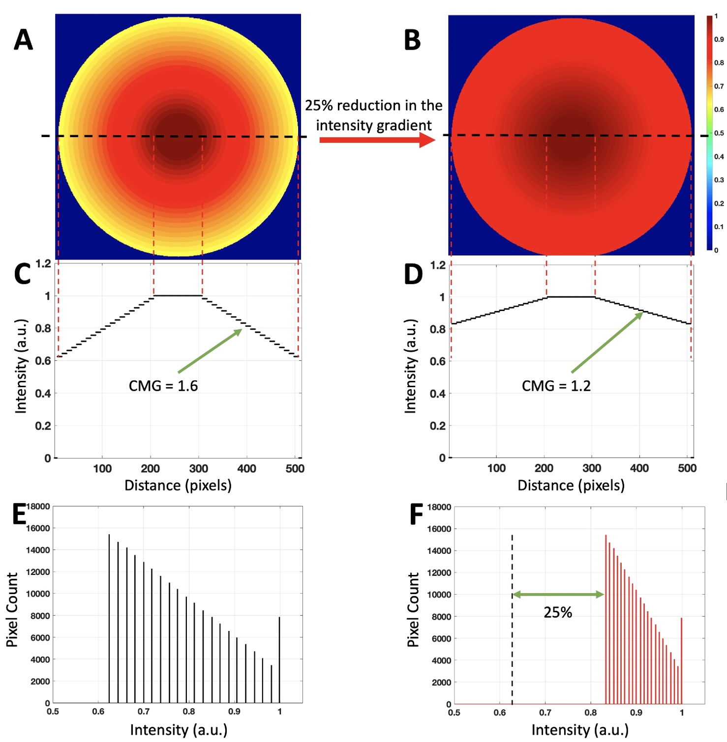
Simulations: To evaluate the image histogram response to CMG changes, a digital phantom was simulated. It consisted of concentric disks, the center disk representing the inner medulla and the outermost representing the edge of cortex (Fig. 1 A). The values of the disks were assigned such that they represent a nominal CMG of 1.6 (Fig. 1 C). A second similar phantom was generated (Fig. 1B) with a CMG of 1.2 to simulate a 25% reduction in the CMG (Fig. 1D). The histograms of the two were then computed.In vivo study design: Two healthy participants fasted 8 hours before the study visit. The study visit included: a baseline proton and sodium MRI, water-load (ingestion of 15 mL of water per one kilogram of body weight), and proton and sodium images were collected together 3 times at 30-minute intervals starting at one hour after water ingestion. Spot urine samples were also collected at the end of each sodium acquisition to determine maximal urine dilution time point.
MRI Acquisition: MRI experiments were performed using a 3 Tesla scanner (Siemens Biograph mMR). Proton images were acquired using the body coil. A custom-built flexible transmit/receive two-loop butterfly coil (diameter=18cm, tuning=32.6 MHz) was used for sodium imaging. Participants lied in supine position on MR bed. The sodium coil was centered on the left kidney. To delineate the borders of the kidney, in phase and opposite phase breath-hold dual-echo T1-weighted images were acquired using a 2D gradient-echo sequence with the following parameters: TR 100 msec, the TE opposite phase 1.23 msec and in phase 2.46 msec, slice thickness 4 mm, 25 slices, matrix 256×256; field of view 36×36 cm2, scan time 36 seconds. Sodium images were acquired using a 3D density-adapted radial projection sequence4 (TR=50ms, TE=0.8ms, FOV=36×36 cm2, slab-selective pulse 10cm thick (same orientation and coverage as proton prescription), flip angle 60 degrees, nominal isotropic resolution 4×4×4 mm3, number of projections=11310, acquisition window 25ms, repetitions=1, total scan time=9.5min).
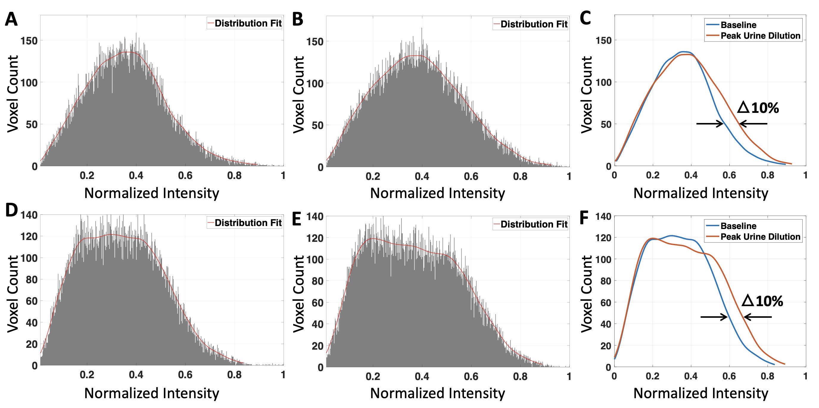
Image reconstruction and analysis: All sodium image reconstruction and analysis were performed in MATALB (R2021a, MathWorks). The sodium signal in the kidneys was isolated and normalized using binary masks produced by drawing outlines of the kidneys on the opposite phase proton images. Sodium histograms of the kidney were then computed. A smooth line was fitted to the histogram distribution. The shift in the fitted lines between baseline and peak urine dilution was measured to quantify the change in CMG due to water load.
Results
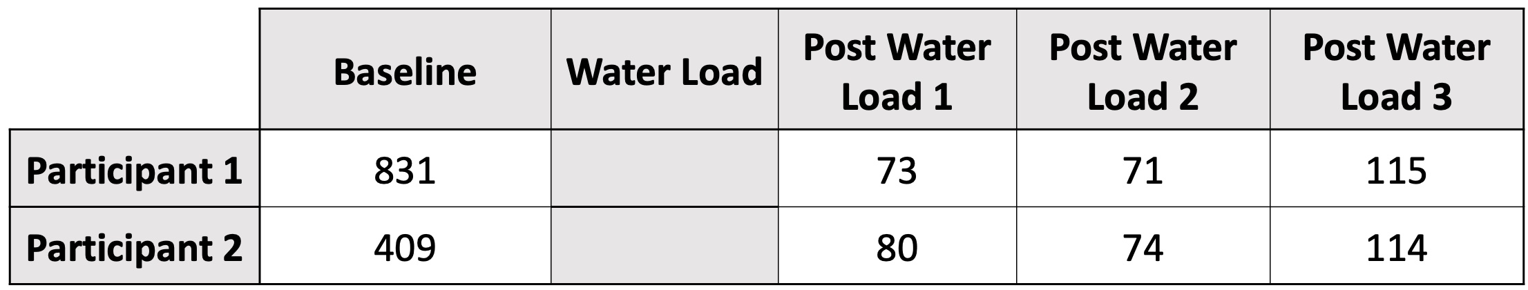
Figure 1. E demonstrates histogram of the phantom with CMG of 1.6. Since the phantom values are normalized to 1, the reciprocal of the leftmost edge of the histogram value (i.e. 1/0.625) represents the CMG. Reducing the CMG by 25%, from 1.6 to 1.2, compressed the image histogram in the second phantom. This resulted in a horizontal shift to the leftmost edge of the histogram by 25%, from 0.65 to 0.833 (Fig. 1 F). Peak urine dilution occurred at the second time point after water load; results are summarized in table 1. The results from normalized sodium image histogram analysis of the two participants showed a maximum of 10% shift in the region where CMG is around 1.6 between the baseline and peak urine dilution as demonstrated in figure 2.Discussion
Simulation analysis shows changes in CMG are directly proportional to the shift in the image histogram. This makes histogram analysis an ideal tool to quantify changes in sodium CMG in the kidney. A previous study3 demonstrated direct correlation between urine osmolality and changes in sodium CMG under water load condition. We used urine osmolality to identify peak urine dilution for histogram comparison. In vivo results indicate a consistent shift of normalized image histogram in both participants as predicted by phantom simulation analysis confirming sodium histogram analysis can quantify the changes in CMG under water load condition.Conclusion
Image histogram analysis helps objectively and quantitatively track changes in sodium CMG in the kidney. This method may help study diuretic drug efficacy in hypertensive patients by quantifying changes in sodium CMG in the kidney.Acknowledgements
No acknowledgement found.References
1. Maril, N., Rosen, Y., Reynolds, G. H., Ivanishev, A., Ngo, L., & Lenkinski, R. E. (2006). Sodium MRI of the human kidney at 3 tesla. Magnetic Resonance in Medicine, 56(6), 1229–1234. https://doi.org/10.1002/mrm.21031
2. Haneder, S., Konstandin, S., Morelli, J. N., Nagel, A. M., Zoellner, F. G., Schad, L. R., Schoenberg, S. O., & Michaely, H. J. (2011). Quantitative and Qualitative 23 Na MR Imaging of the Human Kidneys at 3 T: Before and after a Water Load. Radiology, 260(3), 857–865. https://doi.org/10.1148/radiol.11102263
3. Akbari, A., Lemoine, S., Salerno, F., Marcus, T. L., Duffy, T., Scholl, T. J., Filler, G., House, A. A., & McIntyre, C. W. (2022). Functional Sodium MRI Helps to Measure Corticomedullary Sodium Content in Normal and Diseased Human Kidneys. Radiology, 303(2), 384–389. https://doi.org/10.1148/radiol.211238
4. Nagel, A. M., Laun, F. B., Weber, M. A., Matthies, C., Semmler, W., & Schad, L. R. (2009). Sodium MRI using a density-adapted 3D radial acquisition technique. Magnetic Resonance in Medicine, 62(6), 1565–1573.
Figures