Synopsis

Keywords: Quantitative Imaging, Myocardium

Linear subspace-based models are a powerful method for reconstruction in quantitative magnetic resonance imaging (qMRI). Compared to nonlinear model-based reconstructions, they are computationally more efficient and avoid partial volume effects. Both methods have not yet been compared with respect to myocardial T₁ mapping using single-shot inversion-recovery radial FLASH. This work quantitatively compares the two methods for different regularization parameters. Reconstruction quality and T₁ maps of both methods are comparable.

Introduction

Linear subspace-based models are a powerful method for $$$T_1$$$ and $$$T_2$$$ mapping in MRI.^1-3 Combined with non-Cartesian trajectories^4-6, they provide an efficient tool for quantitative MRI (qMRI). In qMRI, correlations of signal evolution and underlying MR parameters (such as $$$T_1$$$, $$$T_2$$$) of different tissues can often be approximated in a low dimensional subspace. Constrained by the selected basis functions, a linear reconstruction can be performed to estimate the signal evolution, followed by pixel-wise fitting to estimate quantitative maps.
Here, we compare these methods with respect to myocardial $$$T_1$$$ mapping.

Data Acquisition

$$$T_1$$$ mapping is accomplished with a single-shot inversion-recovery (IR) radial FLASH sequence: following a single, non-selective inversion pulse, data is continuously acquired using the FLASH readout. Measurements have been performed on eight volunteers with three repetitive scans each. To avoid motion effects of the systolic contraction and expansion, data from the diastolic phase is retrospectively selected for $$$T_1$$$ mapping.⁵ The myocardium is manually segmented according to Cerqueira et al.⁷. The data was acquired on a 3 T Scanner (Magnetom Skyra, Siemens Healthineers, Erlangen, Germany). A tiny golden angle (18.71°)⁸ was used for radial sampling. Temporal binning was used to reduce computational demand. In this study, 17 spokes were binned to create a single k-space frame with a temporal resolution of 45 ms. According to the subjects’ heart rates, the resulting number of k-space frames were 48 ± 9, range 33–57. Single-shot myocardial $$$T_1$$$ maps of the mid-ventricular slices were acquired at a nominal in-plane resolution of 1.0 × 1.0 mm² and 8 mm slice thickness using a FOV 256 × 256 mm² in combination with a resolution of 512 complex data points per radial spoke (two-fold oversampling). Other parameters were TR/TE = 2.67/1.67 ms, nominal flip angle 6°, bandwidth 850 Hz/pixel and total acquisition time 4 s.⁶

Subspace Reconstruction

The magnetization signal $$$M(t)$$$ for IR-FLASH can be expressed as ^9,10 $$\begin{aligned}M(\boldsymbol{r})=M_{SS}(\boldsymbol{r}) -(M_{SS}(\boldsymbol{r})+M_0(\boldsymbol{r}))\exp{-\frac{t}{T_1^\star(\boldsymbol{r})}}&&(1)\end{aligned}$$ with the steady-state magnetization $$$M_{SS}$$$, the equilibrium magnetization $$$M_0$$$ and the effective $$$T_1$$$ time $$$T_1^\star$$$. Based on equation (1), a dictionary of representative signal curves is simulated by varying $$$T_1^\star$$$ and $$$M_{SS}$$$ values as described in ⁶. As these signal evolutions are highly correlated, a good representation can be achieved using a small number of basis functions $$$B_s(t)$$$, i.e. in a low dimensional linear subspace. Basis functions are obtained by performing singular value decomposition. (Figure 1) Here, four coefficients are used for subspace-based reconstructions.
Signal curves $$$t \rightarrow M(x,t,\boldsymbol{r})$$$ to can be estimated as a linear combination of subspace coefficients $$$a_s$$$ and basis functions $$$B_s$$$:$$\begin{aligned}M(x,t,\boldsymbol{r}) \approx \sum_s a_s(\boldsymbol{r}) B_s(t)&&(2)\end{aligned}$$A regularized inverse problem can be solved for the coefficient maps $$$\boldsymbol{x}$$$ given the k-space data $$$\boldsymbol{y}$$$¹¹:
$$\begin{aligned}\hat a=\underset{a}{\operatorname{argmin}}\lVert\mathcal{PFCB}a-\boldsymbol{y}\rVert_2^2+\mathcal{R}(a)&&(3)\end{aligned}$$ $$$\mathcal{B}$$$ is the multiplication of the coefficient maps with the subspace basis, $$$\mathcal{C}$$$ is the multiplication with the coil sensitivity maps (CSM)s, $$$\mathcal{F}$$$ is the Fourier transform, $$$\mathcal{P}$$$ is the projection to the sampling pattern and $$$\mathcal{R}$$$ is a regularization term. The data is regularized with a locally low-rank regularization with spatial decimation. The regularization parameter was chosen to have a good balance between image details and model accuracy. (Figure 2) All reconstruction steps were performed in BART¹², which features a very efficient implementation of subspace-based reconstructions for non-Cartesian MRI.
Given the coefficient maps $$$a$$$, the signal evolution is obtained by $$$\mathcal{B}a$$$, which in turn is fitted pixel-wise to the signal model to obtain the $$$T_1$$$ map. For more details, refer to the review in ⁶.

Nonlinear Model-based reconstruction

The reference method used in this work, is a sparsity constrained, nonlinear model-based reconstruction⁵, which estimates model parameters $$$x_p=(M_{SS}, M_0, R_1^\star)^T$$$ and coil sensitivity maps $$$x_c=(c_1,...,c_n)^T$$$ directly from k-space:$$\begin{aligned}\hat x =\underset{x}{\operatorname{argmin}}\lVert F(x)-y\rVert _2^2+\alpha R(x_p)+\beta Q(x_c)&&(4)\end{aligned}$$A detailled explanation can be found in $$$^{5}$$$.

Results

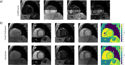
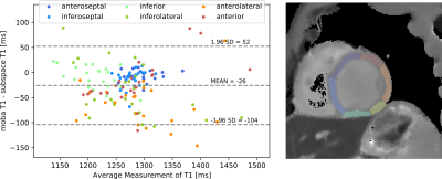
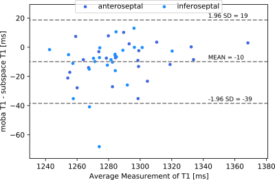
Synthetic images are created for different inversion times, using the coefficient maps of the linear subspace method and the parameter maps of the model-based reconstruction. (Figure 3) In agreement with results for $$$T_1$$$ mapping in the brain$$$^{6}$$$, synthesized images and $$$T_1$$$ maps of the nonlinear method have slightly less noise and better sharpness.
Figure 4 shows the comparison between the $$$T_1$$$ values of linear subspace-based and nonlinear model-based reconstruction with a Bland-Altman plot. $$$T_1$$$ values in the myocardial septum have a mean difference of 10 ms and a standard deviation of 15 ms. (Figure 5)

Discussion and Conclusion

In the $$$T_1$$$ maps obtained with linear subspace-based reconstruction, pixels in the blood pool of right and left ventricle show errors, as the Look-Locker model is violated due to blood flow.
$$$T_1$$$ values obtained from subspace-based reconstructions differ somewhat from values obtained with model-based reconstruction ($$$p<10^{-5}$$$). Further analysis is warranted to examine the larger deviations in the lateral sections of the myocardium.

Acknowledgements

We acknowledge funding by the "Niedersächsisches Vorab" funding line of the Volkswagen Foundation and the Sonderforschungsbereich (SFB) 1456 with project 432680300.