Synopsis

Keywords: Low-Field MRI, Electromagnetic Tissue Properties

Electric conductivity depends on the frequency of the probing electric field. The impact of the frequency differs between human tissue types, e.g., it is lower for body fluids than for cellular tissue types. The upcoming mid-field systems suggest to investigate this frequency dependence with MRI. This study investigated two phantoms, with and without cellular structure, to explore the frequency dependence of conductivity using “Electrical Properties Tomography”. The conductivity results obtained at three different Larmor frequencies were used to estimate the conductivity at lower frequencies in the range of kHz as required for, e.g., EEG source localization.

Introduction

Electric conductivity depends on the frequency of the probing electric field. The impact of the frequency differs between human tissue types: it is lower for body fluids than for cellular tissue types, where α/β/γ/δ-dispersion has been described for different frequency regimes ¹. With the upcoming mid-field systems, it becomes possible to investigate this frequency dependence with MRI ². This study investigated two phantoms, with and without cellular structure, to explore the frequency dependence of conductivity using “Electric Properties Tomography” (EPT) ³. A deeper understanding of this topic might be useful to estimate conductivity at frequencies in the range of kHz as required for, e.g., EEG source localization.

Methods

A water melon was used as soft tissue model and compared with a saline phantom (2g NaCl / liter H2O) at B₀=0.6T, 1.5T, and 3.0T MRI systems (Philips Healthcare, Best, Netherlands). A steady-state free-precession (SSFP) sequence (voxel 2x2x2 mm³, TR/TE=2.5/1.25ms, flip angle(0.6T/1.5T/3.0T)=60°/30°/30°, NSA(0.6T/1.5T/3.0T)=4/2/2) was applied at all fields strengths, and a DREAM sequence ⁴ (voxel 4x4x8 mm³, imaging angle 10°, STEAM angle 50°, TR/TE1/TE2(1.5T)=8.8/2.7/4.6ms, TR/TE1/TE2(3T)=4.4/1.6/2.3ms) for the two higher field strengths. EPT reconstructions were performed as in ⁵ to obtain conductivity at 25 MHz, 64 MHZ, and 128 MHz from the SSFP phase (representing B₁ phase) and for B₀=1.5T and B₀=3.0T additionally taking the B₁ magnitude from DREAM into account (i.e., constant B₁ magnitude assumed for B₀=0.6T).
The conductivity averaged over 3x3x3cm³ in the melon’s center (apart from seeds) was used as input for the simplified Cole-Cole-model ⁶ to estimate the melon’s conductivity corresponding to the range of kHz. The obtained value was compared with the melon’s conductivity obtained with an impedance analyzer (4294A, Agilent, USA) at 1kHz. Conductivity values of the saline were compared with the model of Stogryn ⁷.

Results

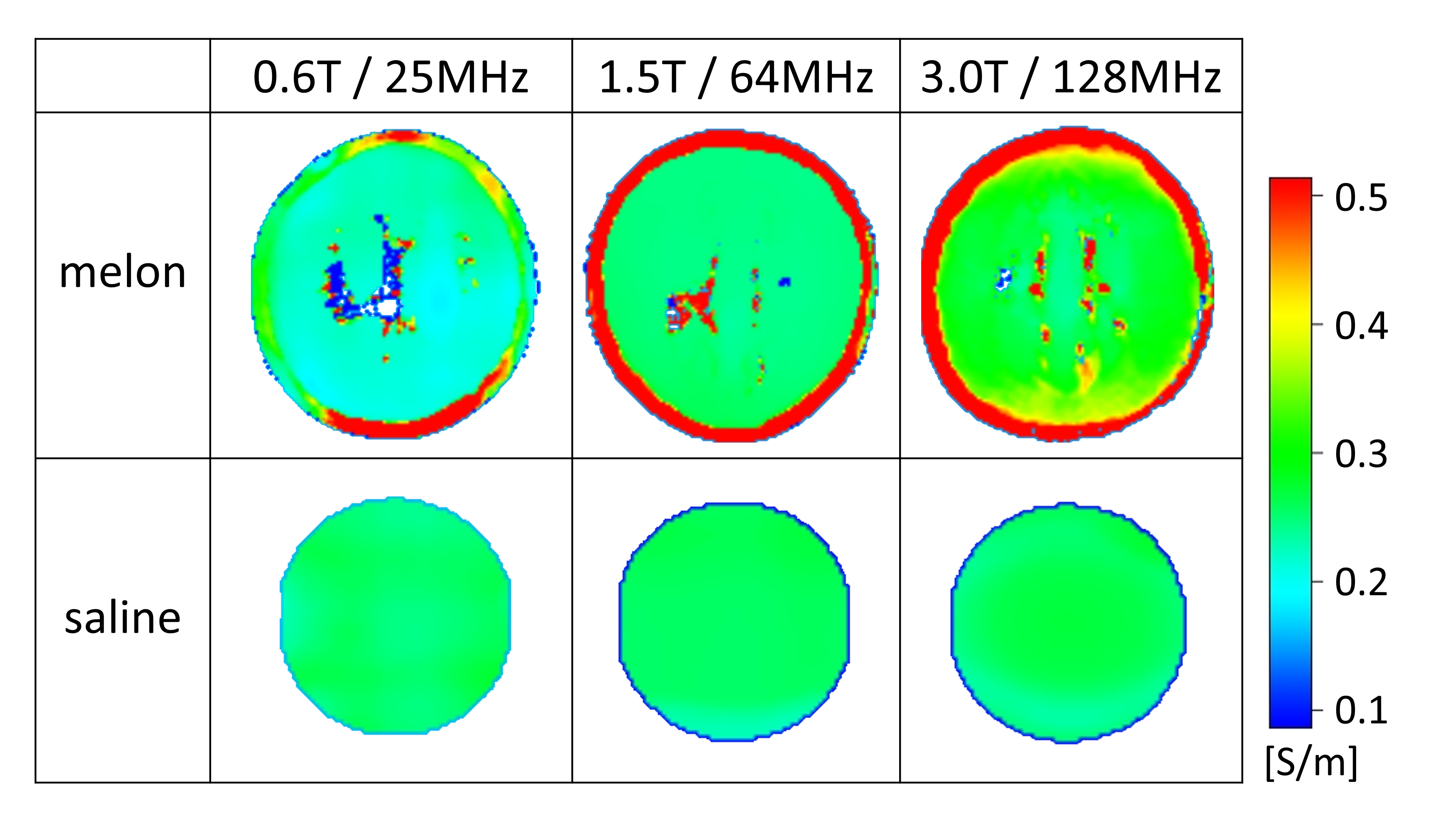
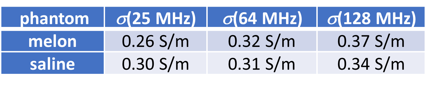
Conductivity maps of the two phantoms are shown for the three different field strengths in Fig. 1. A table with mean conductivities found in these experiments are given in Fig. 2. Using the mean conductivity values for the melon as input for the simplified Cole-Cole model ⁶ yielded 0.04 S/m. The conductivity of the melon as measured with the impedance analyzer at 1 kHz was 0.03 S/m.

Discussion and Conclusion

The cellular substance of the water melon revealed a clear frequency dependence, which was in line with the simplified Cole-Cole model ⁶. It thus confirmed that multi-RF frequency conductivity measurements can be used to estimate conductivity at lower frequencies in the range of kHz as required for, e.g., EEG source localization. On the other hand, no clear frequency dependence could be identified for the saline phantom, as expected from literature ⁷. A conductivity change of only 3% across the investigated frequency range is described for the saline concentration used in this study, which is below the sensitivity of the applied experimental setup. The study shall be extended to in vivo measurements to examine the frequency dependence of different tissue types.

Acknowledgements

The authors would like to thank Christoph Leussler for supporting the measurements with the impedance analyzer.

References

1. Gabriel S et al., The dielectric properties of biological tissues: III. Parametric models for the dielectric spectrum of tissues. Phys Med Biol. 1996;41:2271

2. Iyyakkunnel S, Bieri O, Conductivity mapping at 0.55 T with balanced steady state free precession. Proc. ISMRM 2022;30:2913.

3. Katscher U et al., Electric properties tomography: Biochemical, physical and technical background, evaluation and clinical applications. NMR Biomed. 2017;30:3729

4. Nehrke K et al., DREAM - a novel approach for robust, ultrafast, multislice B1 mapping. Magn Reson Med. 2012;68:1517

5. Tha KK et al., Noninvasive electrical conductivity measurement by MRI: a test of its validity and the electrical conductivity characteristics of glioma. Eur Radiol. 2018;28:348

6. Katscher U et al., Estimation of low frequency conductivity from Larmor frequency conductivity. Proc. ISMRM 2019;27:695.

7. Stogryn A, Equations for calculating the dielectric constant of saline water, IEEE Trans Microwave Theory Tech 1971;19(8):733–736.