1587
Balanced steady-state free precession imaging and associated rapid relaxation time mapping on a point-of-care 46 mT Halbach MRI scanner
Chloé Najac1, Florian Birk2,3, Tom O’Reilly1, Klaus Scheffler2,3, Andrew Webb1, and Rahel Heule2,3,4
1C.J. Gorter MRI Center, Department of Radiology, Leiden University Medical Center, Leiden, Netherlands, 2Department of High-Field Magnetic Resonance, Max Planck Institute for Biological Cybernetics, Tübingen, Germany, 3Department of Biomedical Magnetic Resonance, University of Tübingen, Tübingen, Germany, 4Center for MR Research, University Children's Hospital, Zurich, Switzerland
1C.J. Gorter MRI Center, Department of Radiology, Leiden University Medical Center, Leiden, Netherlands, 2Department of High-Field Magnetic Resonance, Max Planck Institute for Biological Cybernetics, Tübingen, Germany, 3Department of Biomedical Magnetic Resonance, University of Tübingen, Tübingen, Germany, 4Center for MR Research, University Children's Hospital, Zurich, Switzerland
Synopsis
Keywords: Low-Field MRI, Data Acquisition
Point-of-care imaging with low-field MRI (<0.1T) is a potential game changer for low-income countries and the intensive care unit. The main challenge is the low SNR. Balanced steady-state free precession (bSSFP) sequences are fast and SNR-efficient. However, bSSFP is very sensitive to B0 inhomogeneities resulting in banding artifacts. We evaluated the feasibility of using bSSFP on our 46 mT MRI scanner. By acquiring 17 bSSFP datasets with linearly increasing frequency offsets (from 0 to 1/TR), we could reconstruct banding-free maximum-intensity images as well as F0 and F-1 SSFP configurations, which we employed for rapid relaxation time mapping.Introduction
Development of low-field MRIs (with B0<0.1T) for point-of-care (POC) applications has recently become increasingly widespread1. The reduced cost and improved portability drastically increase their accessibility compared to conventional systems. However, low-field brain images suffer from low SNR and poor tissue contrast2. The balanced steady-state free precession (bSSFP) imaging sequence is fast, offers high SNR, and produces a T2/T1-weighted image contrast3. However, bSSFP is very sensitive to B0 inhomogeneities (ΔB0), which lead to banding artifacts3. Banding-free images can be achieved by acquiring multiple images using RF phase-cycling increments or frequency offsets3. Although optimized passive and active shimming schemes have been developed to minimize ΔB04, compact low-field permanent MRI systems based on cylindrical Halbach arrays have intrinsically large ΔB0 (~thousands ppm) due to the finite diameter-to-length ratio5 compared to larger low-field fixed location systems on which bSSFP has been implemented6. Here, we wanted to evaluate the potential of bSSFP on our 46mT imaging system.Materials and Methods
Hardware: We used a 46mT Halbach array-based magnet (outer/inner diameter=60/30.1cm, length=49.2cm, weight=111kg), with custom-built RF and Bruker gradient amplifiers and a Magritek Kea2 spectrometer7. Imaging was performed using a solenoid and an elliptical spiral-solenoid head coil2,7.bSSFP implementation: The 3D bSSFP sequence consisted of a train of hard pulses with alternating flip angle (α), following an α/2 ramp preparation (Fig.1A). A zig-zag phase-encode trajectory was used to smoothly sample k-space8 (Fig.1B). To correct for banding artifacts we used a range of equidistant frequency offsets between 0 and 1/TR.
Sequence validation (n=3): 5 tubes were filled with water-based agarose gel (ranging from 0 to 4%) and 2mM copper-sulfate to obtain different T1/T2 ratios (Fig.2A). T2 mapping was performed using a 3D Carr-Purcell-Meiboom-Gill (CPMG) imaging sequence (resolution=3x3x10mm3, TR/echo-spacing=1250/20ms, 10 echoes, acq. time~15min). T1 mapping was performed using 3D inversion recovery (IR) scans with TSE readout (identical resolution, TR/TE/TEeff=1250/14/14ms, ETL=6, inversion times=50/100/150/200/300/400ms, acq. time~15min). A series of 11 bSSFP datasets (identical resolution, TR/TE=16/8ms, acq. time~11x3.4min) were acquired with a flip angle varying from 10º to 170º. Maximum-intensity bSSFP images were reconstructed for each flip angle using 17 frequency offset increments. The signal was averaged over 8 slices and a region-of-interest (5x5 pixels) was defined to extract proton-density (PD), T2, T1 and bSSFP values within each sample (Fig.2/3). BSSFP signal evolution as a function of flip angle was fitted with the theoretical expression3: $$$\frac{M_{SS}}{M_{0}}=\frac{sin(\alpha)}{1+cos(\alpha)+(1-cos(\alpha))*\frac{T_{1}}{T_{2}}}$$$. Optimal flip angle and steady-state level obtained from the fit were compared to values derived from T1/T2 mapping performed with CPMG/IR sequences using the formula3: $$$FA_{optim}=arcos(\frac{\frac{T_{1}}{T_{2}}-1}{\frac{T_{1}}{T_{2}}+1})$$$ and $$$M_{SS}=\frac{1}{2}*M_{0}*\sqrt{\frac{T_{2}}{T_{2}}}$$$.
Brain-like (BrainLo) phantom experiment: BrainLo was built using a 3D printer and filled with different solutions of agarose/copper-sulphate doped-water/deuterated-water to imitate brain tissue relaxation properties (Fig.3A). T2/T1 mapping was performed as described above with (resolution: 2x2x10 mm3, total acq time~10/8 mins for CPMG/IR sequences). bSSFP data (identical resolution, total acq. time~2 mins) were acquired with α=90º. First, the sum of squares, complex sum, magnitude sum, and maximum-intensity images were calculated, neglecting any additional frequency drift during multi-offset series’ acquisition (Fig.4). Secondly, F0 and F-1 modes were retrieved via a Fourier transform of the complex bSSFP frequency response, incorporating the measured frequency drift. Finally, a T2 map was calculated using the F0 and F-1 configurations in an approach similar to MIRACLE relaxometry9-12.
Results and Discussion
Sequence validation: As illustrated in Fig.2A, our samples had T1/T2 ratios ranging from ~1:1 to ~4.7:1. Banding-free maximum-intensity image could be reconstructed (Fig.2B). Fig.3A shows the evolution of the signal as a function of the flip angle. The sample with the lowest and highest T1/T2 ratio shows the highest and lowest signal respectively, which is in agreement with literature3. The optimal flip angle, steady-state signal level and T1/T2 ratio were close to expected values (Fig.3B). Note however, that the fit slightly deviated from data for low flip angle since in this regime, the maximum might not occur in the passband but at different frequency offsets. The steady-state signal at the highest T1/T2 ratio was slightly higher than predicted from the model.Brain-like (BrainLo) phantom: As shown in Fig.4A, GM/WM/CSF compartments had T2 and T1 values measured using conventional techniques which match in vivo values at low-field2. Slight residual banding was observed in each reconstruction, except for the maximum-intensity image (Fig.4B). The cause is probably small drifts in B0 during acquisition. By calculating the difference between each dataset and the first dataset (Fig.5A), we estimated this additional drift, corrected it and produced banding-free F0 and F-1 modes (Fig.5B), which were used to reconstruct the T2 map. The relative T2 values are in the right ratio, but absolute values in WM/GM are ~40% lower than those obtained using the much slower conventional techniques. In future experiments we will investigate whether this is a systematic error, or simply reflects the fact that different acquisition schemes result in different apparent relaxation times.
Conclusion
POC imaging with low-field MRI (B0<0.1T) is a potential game changer for low-income countries and patients in the intensive care unit. However, POC systems have intrinsically low SNR and relatively high ΔB0. We illustrated the feasibility to reconstruct banding-free bSSFP images at 46mT on a portable POC system and to rapidly quantify T2 based on the retrieved F0 and F-1 configurations.Acknowledgements
This project has received funding from Horizon 2020 ERC Advanced PASMAR 101021218, ERC advanced grant SpreadMRI 834940 and the Dutch Science Foundation Open Technology 18981.References
1Saracanie, Front. Phys. (2020) ; 2O’Reilly et al., MRM (2021) ; 3Scheffler et al., Eur Radiol (2003) ; 4O’Reilly et al., ISMRM #63 (2022); 5Koolstra et al., MAGMA (2021); 6Saracanie et al., Sci. Rep. (2015) ; 7O’Reilly et al., MRM (2020); 8Scheffler et al., ISMRM #294 (2003) ; 9Heule et al., MRM (2013) ; 10Welsch et al., MRM (2009) ; 11Heule et al., MRM (2014) ; 12Nguyen et al., MRM (2017)Figures
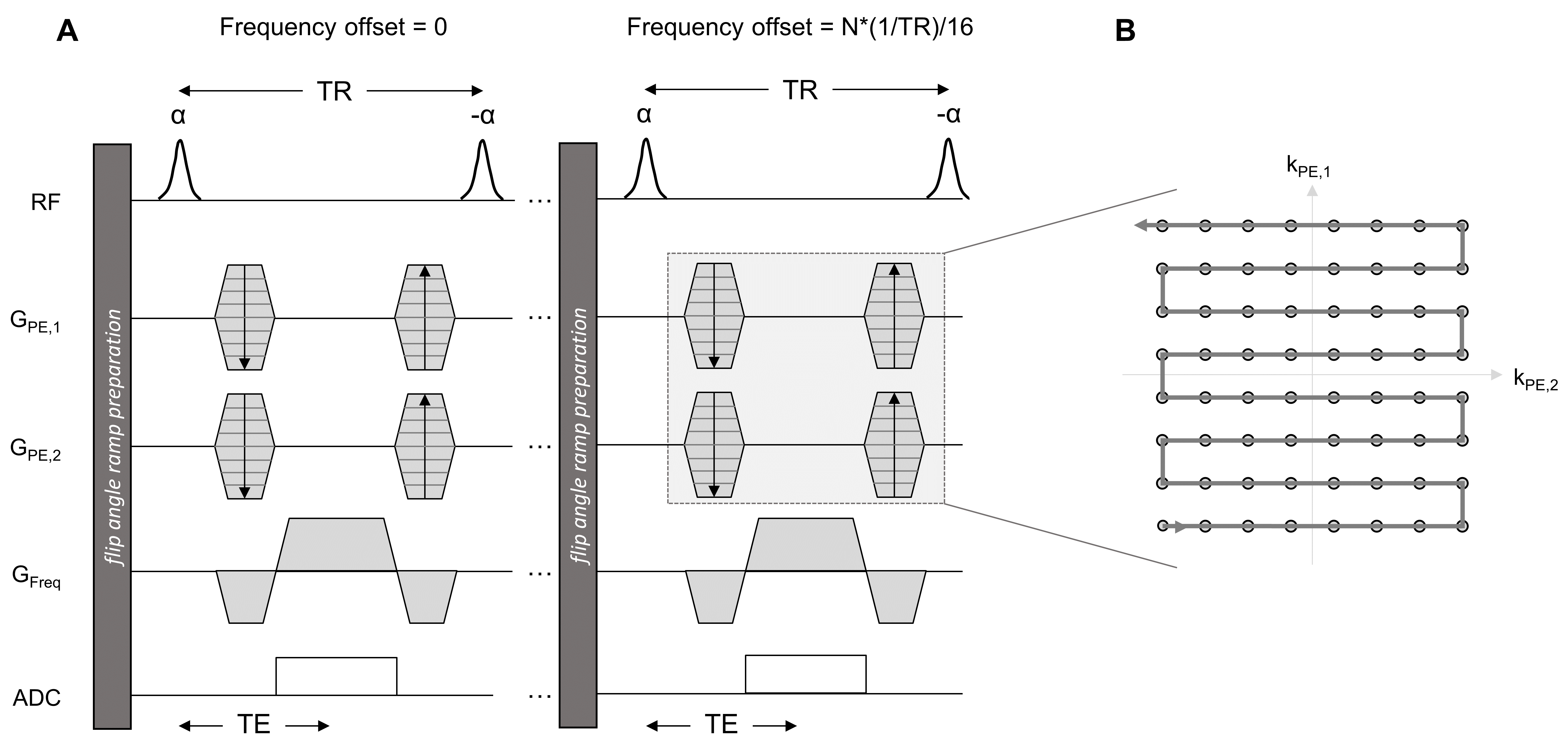
Figure 1 (A) Schematic
representing the implementation of the bSSFP sequence and (B) k-space
trajectory on our point-of-care (POC) 46mT MRI scanner. 17 3D bSSFP datasets
were acquired with frequency offsets ranging from 0 to 1/TR and using a zig-zag
phase-encode trajectory.
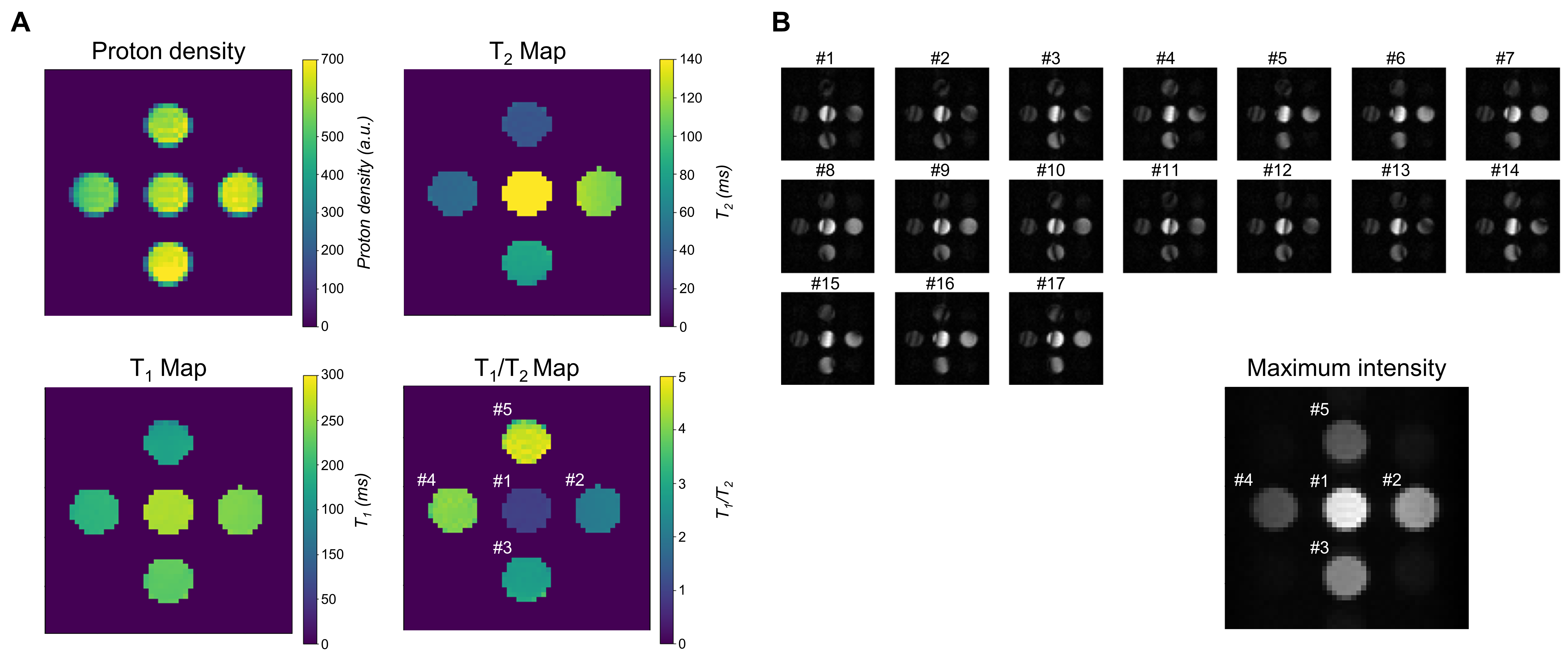
Figure 2 (A) Proton density
(PD), T2 map, T1 map, and T1/T2 ratio
map measured using conventional sequences (CPMG and IR) in our 5-tubes
phantoms. (B) Series of bSSFP images acquired with a flip angle of 90º,
illustrating the banding artifacts and drift of the bands across frequency
offsets. Maximum-intensity image is shown, demonstrating the successful removal
of banding artifacts. Numbers indicate on T1/T2 map and
maximum-intensity image correspond to sample id.
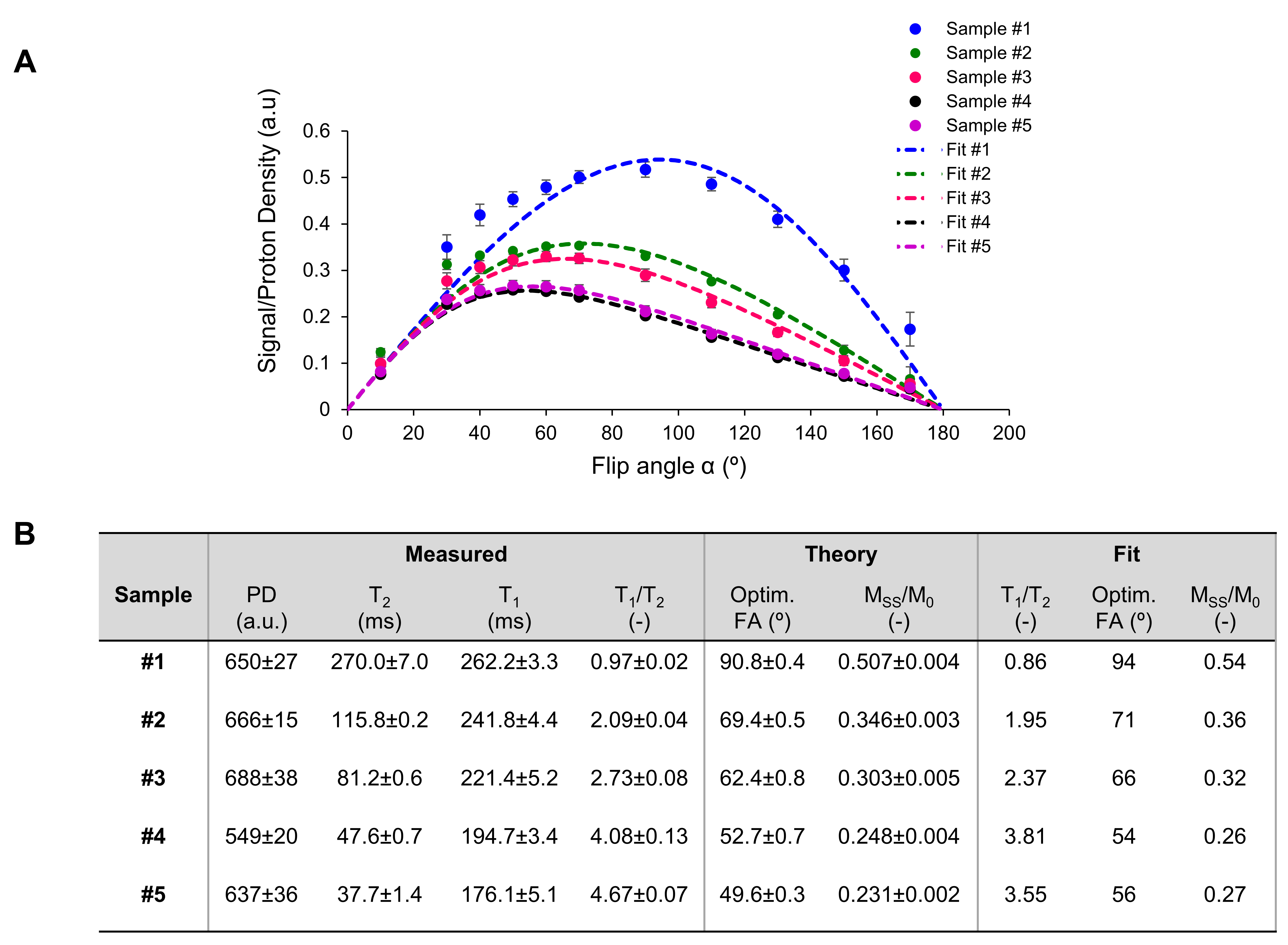
Figure 3 (A) Evolution of the
signal (measured on reconstructed maximum-intensity image and normalized to PD)
as a function of the flip angle of the α RF pulse for all five samples (colored
points). Data from each sample was fitted (dotted lines) with theoretical
expression: $$$\frac{M_{SS}}{M_{0}}=\frac{sin(\alpha)}{1+cos(\alpha)+(1-cos(\alpha))*\frac{T_{1}}{T_{2}}}$$$. (B) Table summarizing the
mean±s.d for measured PD, T2, T1 and T1/T2
as well as theoretical and fitted values for optimal flip angle and
steady-state level for all samples.
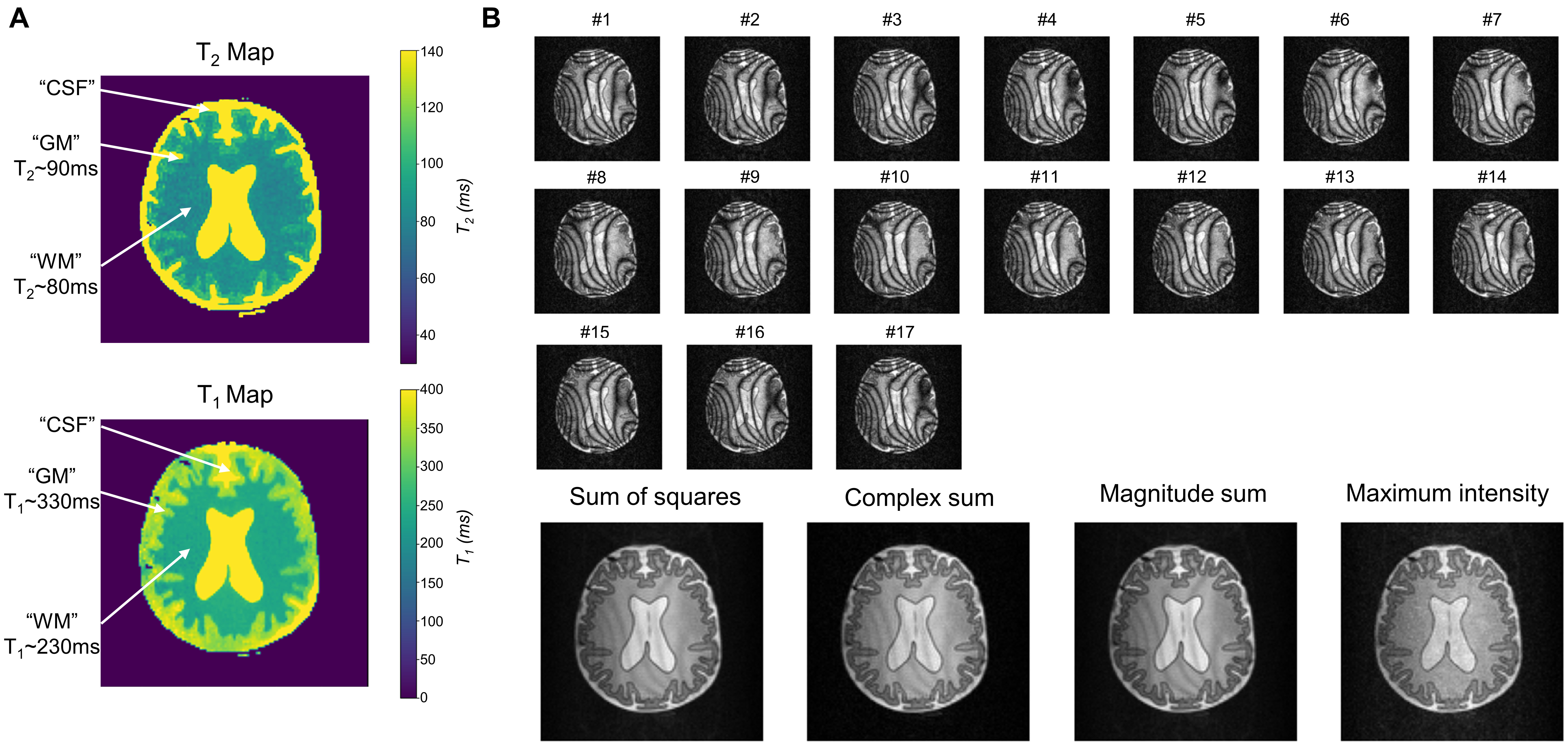
Figure 4 (A) T2 and T1 maps of the
BrainLo phantom obtained with conventional CPMG and IR sequences. (B) Series
of bSSFP images acquired with a flip angle of 90º, illustrating the banding
artifacts and altered positions of the bands at incremental frequency offsets. Slight
residual banding artifacts are observed on the reconstructed sum of squares,
complex sum, and magnitude sum images, whereas a maximum-intensity image was
banding-free.
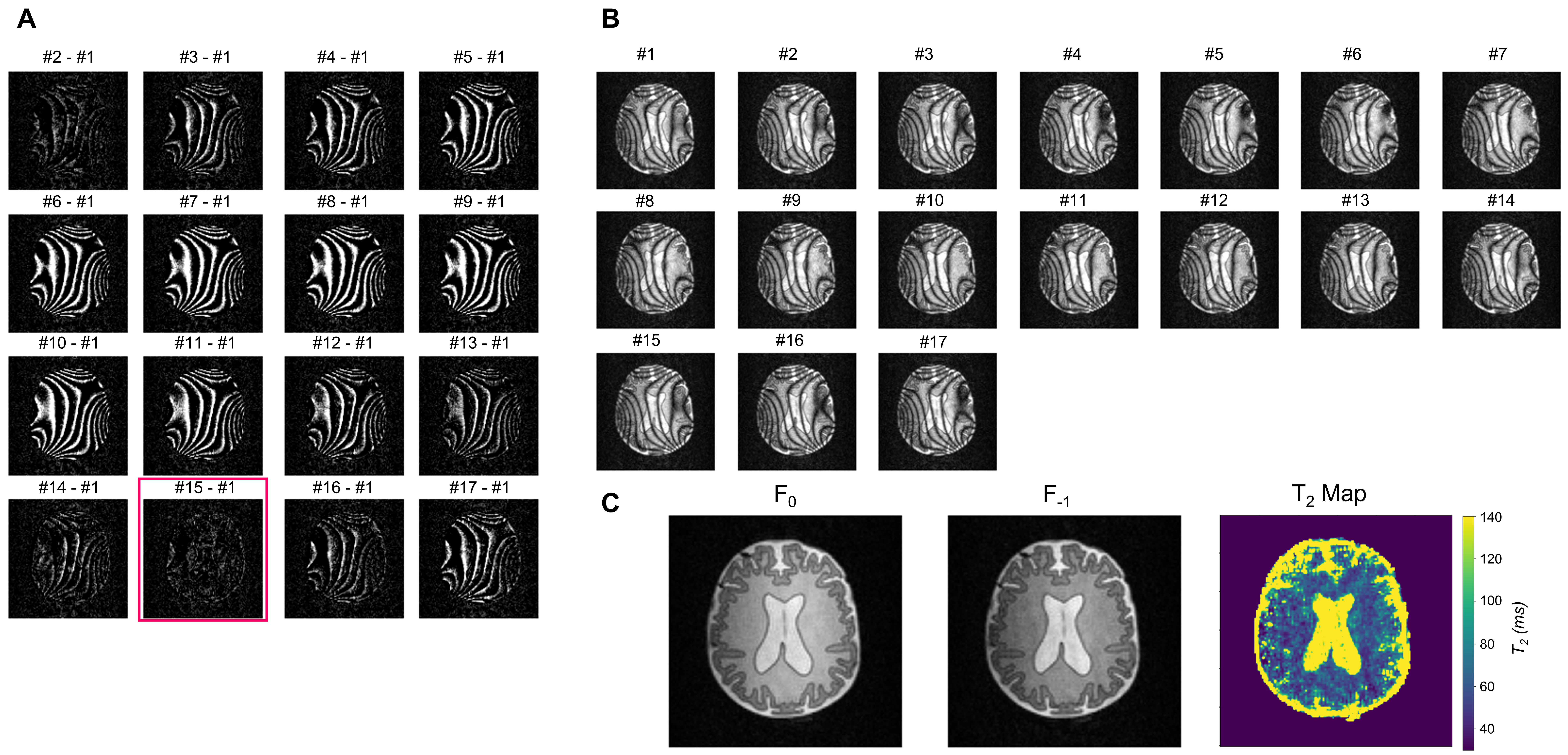
Figure 5 (A) Difference between each
dataset and the first dataset (#1) was calculated to evaluate and (B)
correct for frequency drift during acquisition. Data showed that image #15 was
the closest to image #1 (highlighted with red square). Images #15-17 were
removed from further analysis to avoid oversampling the profile for the Fourier
transform. (C) F0 and F-1 modes and T2
map were reconstructed.
DOI: https://doi.org/10.58530/2023/1587