1556
Controlled Modeling of Cerebrospinal Fluid Flow Artifacts with a Simple Digital Spine Phantom
Daniel V Litwiller1, R Scott Hinks2, Ajeetkumar Gaddipati3, Trevor Kolupar3, and Suchandrima Banerjee4
1GE Healthcare, Denver, CO, United States, 2GE Healthcare, Albuquerque, NM, United States, 3GE Healthcare, Waukesha, WI, United States, 4GE Healthcare, Menlo Park, CA, United States
1GE Healthcare, Denver, CO, United States, 2GE Healthcare, Albuquerque, NM, United States, 3GE Healthcare, Waukesha, WI, United States, 4GE Healthcare, Menlo Park, CA, United States
Synopsis
Keywords: Spinal Cord, Artifacts
Robust spine imaging with conventional fast spin echo remains a clinical challenge due to motion artifacts from multiple sources. Flow artifacts from cerebrospinal fluid can be especially problematic for assessments of the spinal cord itself. In addition, judging the effectiveness of various protocol modifications can be challenging in vivo due to the stochastic nature of the relationship between image timing and the cardiac cycle. In this work, we present results of a simple digital spine phantom that can be used in the controlled evaluation of strategies to mitigate artifacts from CSF flow.Introduction
Although spine imaging represents the largest procedural volume for MRI, consistency in spinal cord image quality remains a challenge in routine clinical imaging. Cervical and thoracic spine imaging is particularly challenging due to motion artifacts from swallowing, breathing, and pulsatile cerebrospinal fluid (CSF) flow. Flow artifacts from CSF can be especially problematic for assessments of the spinal cord itself, and the overall curvature of the anatomy tends to limit the efficacy of flow compensation, when applied in a single direction. In addition, the emergence of deep learning-based image reconstruction has laid bare, in many cases, the presence of even subtle, underlying CSF flow artifacts (Figure 1), raising the profile of this issue. In spite of its overall its sensitivity to motion and flow, however, conventional multi-shot fast spin echo (FSE, aka TSE) remains the preferred clinical sequence for spine imaging, versus alternatives such as PROPELLER (MultiVane, Blade, etc.). Efforts to evaluate protocol modifications are often hampered in vivo due to the random and asynchronous nature of the acquisition relative to the cardiac cycle. Therefore, the purpose of this work was to develop a simple, digital spine phantom that could be used in the controlled evaluation of CSF flow artifacts with respect to current approaches and future technical development efforts.Methods
We developed a parameterized, digital spine phantom consisting of simplified spinal anatomy in the sagittal orientation, including spinal cord, CSF, and background tissue components (Figure 2), with associated tissue parameters (Table 1). In addition, the model includes a dynamic displacement component, applied via a unit-velocity map (Figure 2d, e) to the CSF regions of the phantom (Figure 2f), and parameterized by peak velocity, heart rate, and "quiescent fraction", corresponding to the quiescent portion of the cardiac cycle1. Together with a standard sagittal, T2-weighted FSE protocol, phase encode scheme, and associated gradient waveforms (SIGNA Premier, GE Healthcare, Waukesha, WI), we used this phantom to simulate artifacts due to phase errors accumulated by the spin echo component of the flowing CSF, under several different scenarios, and a wide range of timings (Table 1), in order to produce a statistical representation of associated image errors2,3. Time-of-flight and non-CPMG effects were not considered. Imaging scenarios modeled included FOV angle, phase encode shuffling, complex signal averaging, and two-dimensional flow compensation. All scenarios used flow compensation in the readout direction, and a maximum CSF velocity of 10 cm/s. Normalized root mean squared error (NRMSE) and the structural similarity index metric (SSIM) were computed for the spinal cord region of the simulated images, excluding artifacts manifesting in the CSF and/or background tissue.Results
The results of 3,125 simulations are summarized in the box plots in Figure 3, showing NRMSE and SSIM measurements for the spinal cord region (only) of the phantom. Outliers (above 1.5 times the intraquartile range) are shown in red, and observed to decrease in severity as the scenarios progress from left to right. Figure 4 contains representative images taken from the upper bound of the NRMSE sample for each imaging scenario, along with a motion-free reference (Figure 4f). Image profiles are also presented in Figure 4g, demonstrating differences in artifact level for the imaging scenarios presented.Discussion
As a whole, the statistical representation of the simulations presented in Figure 3 reflect the significant variations in image quality encountered in clinical spine imaging. From a clinical standpoint, and the need to avoid non-diagnostic image quality, the distribution of outliers is of greatest interest, and these results predict that two-dimensional flow compensation (e), followed by complex averaging (d), will produce the most robust results of the scenarios considered. Interestingly, phase encode shuffling (c) appears to have an overall negative impact on these image quality metrics, versus its conventionally-encoded counterpart (b). The median performance of the angled-FOV scenario (a) is comparable to the less-angled counterparts, but occasionally produces highly-corrupted images that are not desirable. NRMSE & SSIM are in relative agreement, though SSIM shows higher variability (i.e. fewer outliers in scenarios a-d), and, as always, it will be beneficial to understand how these measurements compare to scoring by a trained, human reader. The simplicity of this model has allowed us to simulate a large number of images, but the utility of the model could be increased by adding complexity, and incorporating additional effects, such as TOF, non-CPMG, accelerated imaging, and echo spacing impacts due to flow compensated phase encode gradient waveforms. These improvements are left as future work.Conclusion
We have developed a digital spine phantom that is capable of simulating CSF flow artifacts under a wide variety of conditions, and may prove useful in the ongoing assessment and future development of various strategies to enable robust and reliable clinical imaging of the spinal cord.Acknowledgements
No acknowledgement found.References
- Bhadelia RA, Bogdan AR, Wolpert SM. Analysis of cerebrospinal fluid flow waveforms with gated phase-contrast MR velocity measurements. AJNR Am J Neuroradiol. 1995 Feb;16(2):389-400.2.
- Nishimura DG, Jackson JI, Pauly JM. On the nature and reduction of the displacement artifact in flow images. Magn Reson Med. 1991 Dec;22(2):481-92.
- Hinks RS, Constable RT. Gradient moment nulling in fast spin echo. Magn Reson Med. 1994 Dec;32(6):698-706.
Figures
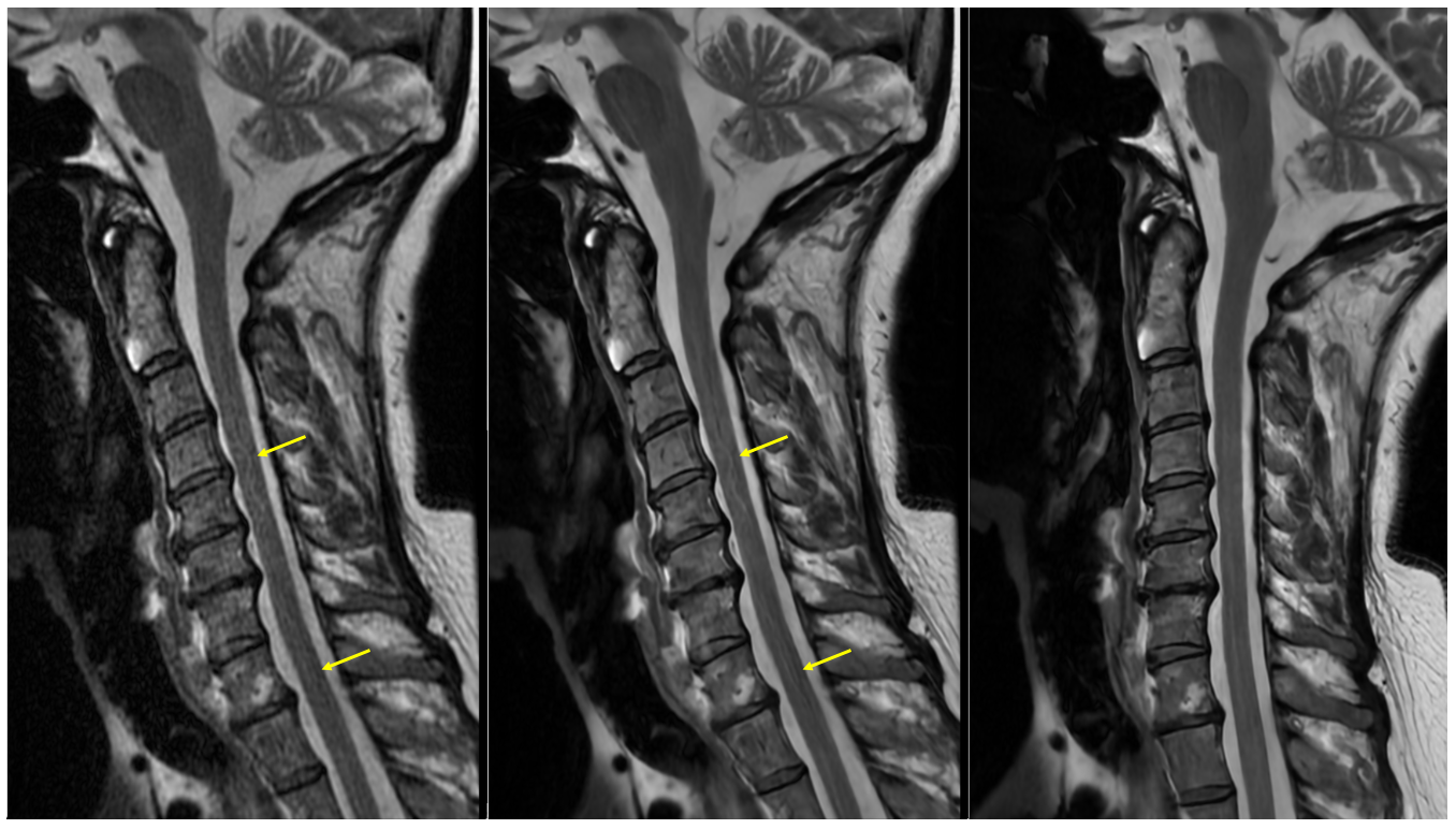
Figure 1. Anecdotal sagittal T2 FSE imaging example. Conventional reconstruction of a straight sagittal acquisition (left), deep learning (DL)-based reconstruction of the straight sagittal acquisition (middle), and DL-based reconstruction of a rotated acquisition (right). DL-based image reconstruction reveals underlying flow artifacts that are mitigated, in this example, by rotating the acquired field of view until the phase encode direction is roughly aligned to the spinal cord, which has been intentionally straightened during patient positioning.
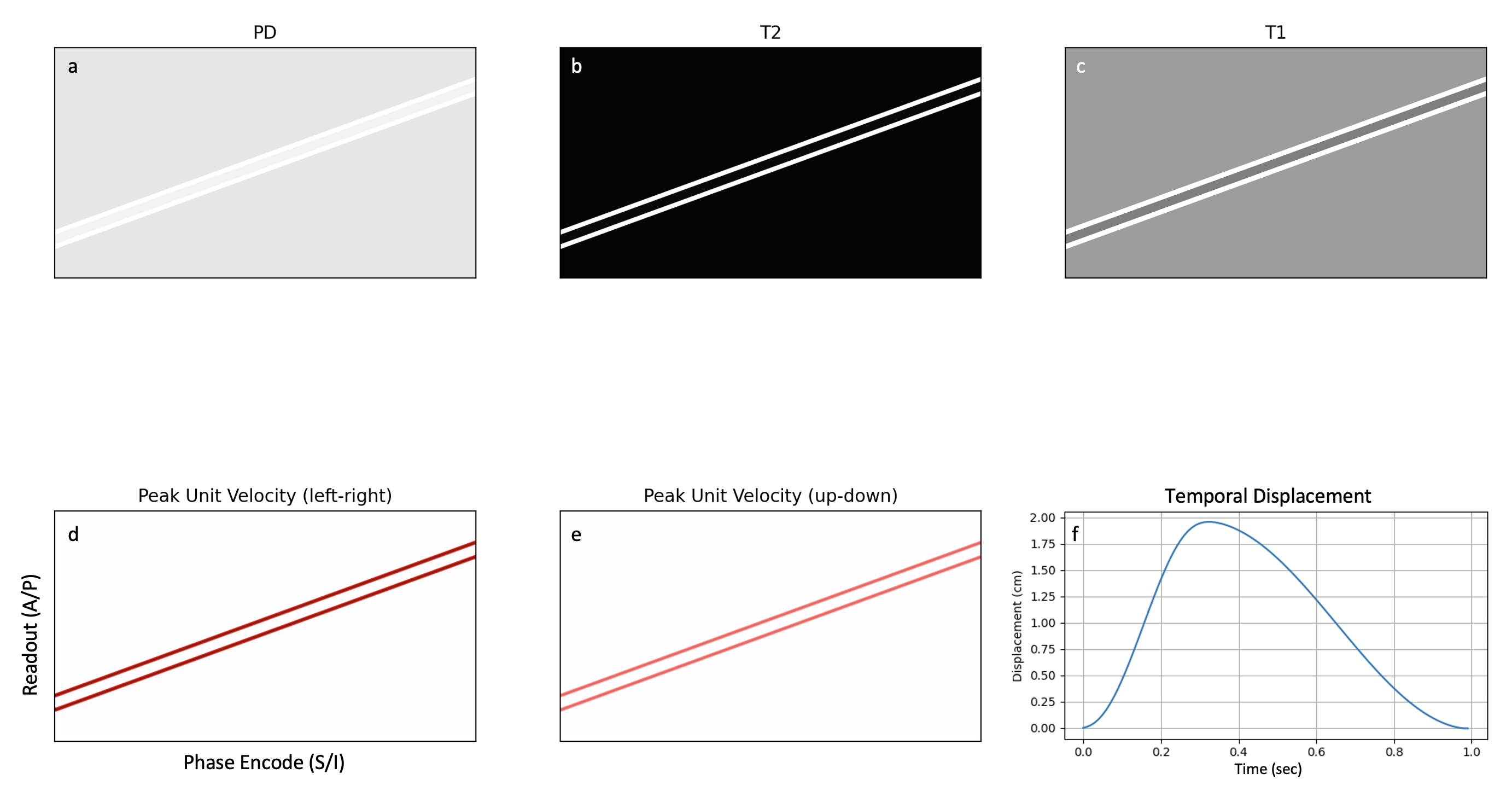
Figure 2. Digital spine phantom in the sagittal orientation, illustrating spinal cord, CSF, and tissue background (muscle) components, with anatomical S/I pointing in the L/R direction. The top row contains PD/T2/T1 maps (see Table 1 for full tissue parameters). The bottom row contains peak in-plane unit-velocity maps for CSF, and an arbitrary temporal CSF displacement curve for a peak CSF velocity of 10 cm/s, a heart rate of 60 beats per minute, and a "quiescent fraction" of 0.7, which corresponds to the right side of the displacement curve.
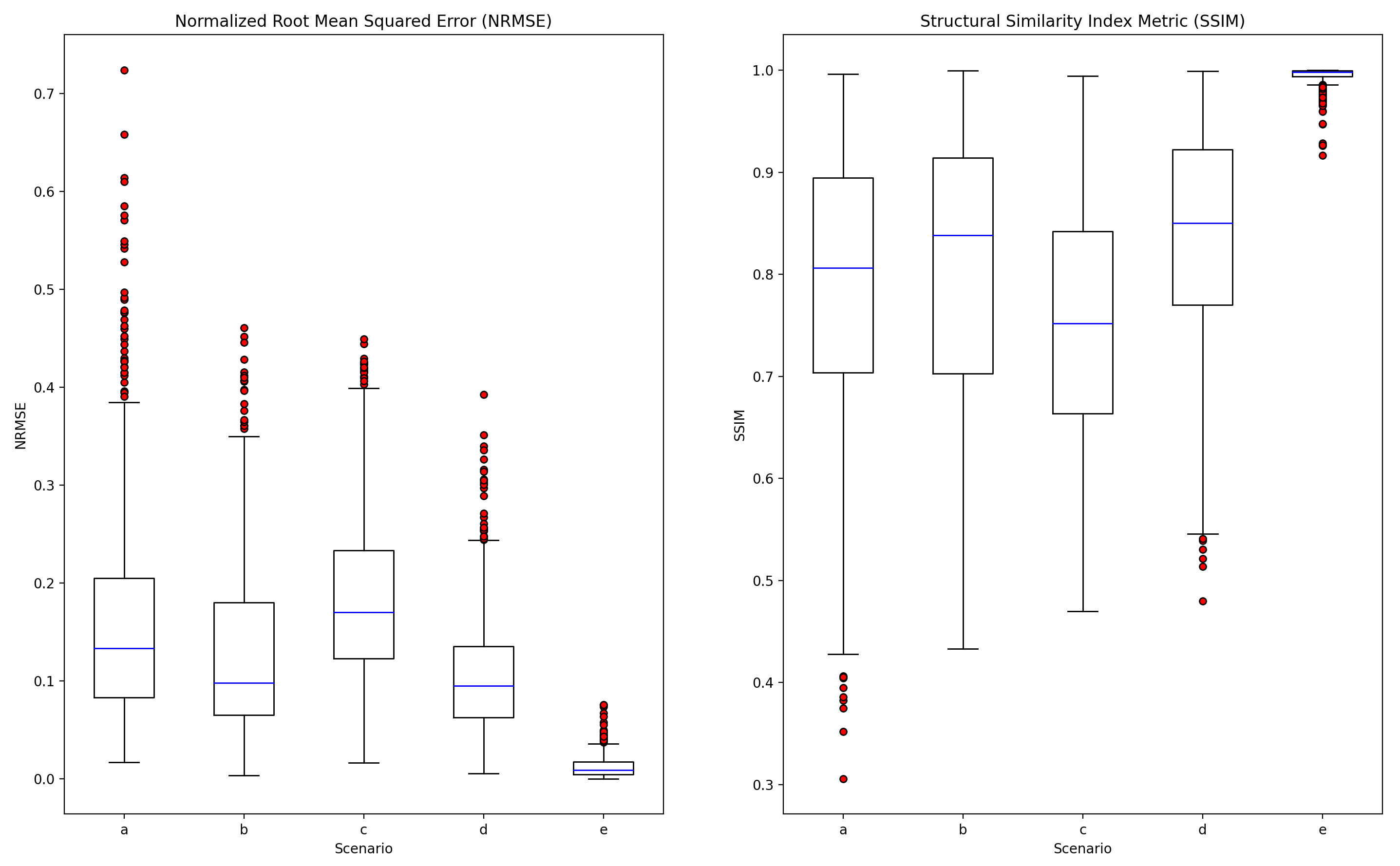
Figure 3. Summary of simulation results. Box and whisker plots of NRMSE and SSIM, computed on the cord region (only) of the reconstructed image, for the five scenarios described in Table 1, a) 15-degree FOV angle, b) 5-degree FOV angle, c) view shuffling, d) two complex averages, e) flow compensated phase encode waveform (S/I). High-error outliers are depicted in red, with the upper NRMSE (and lower SSIM) bound on each dataset defined as 1.5 times the intraquartile range.
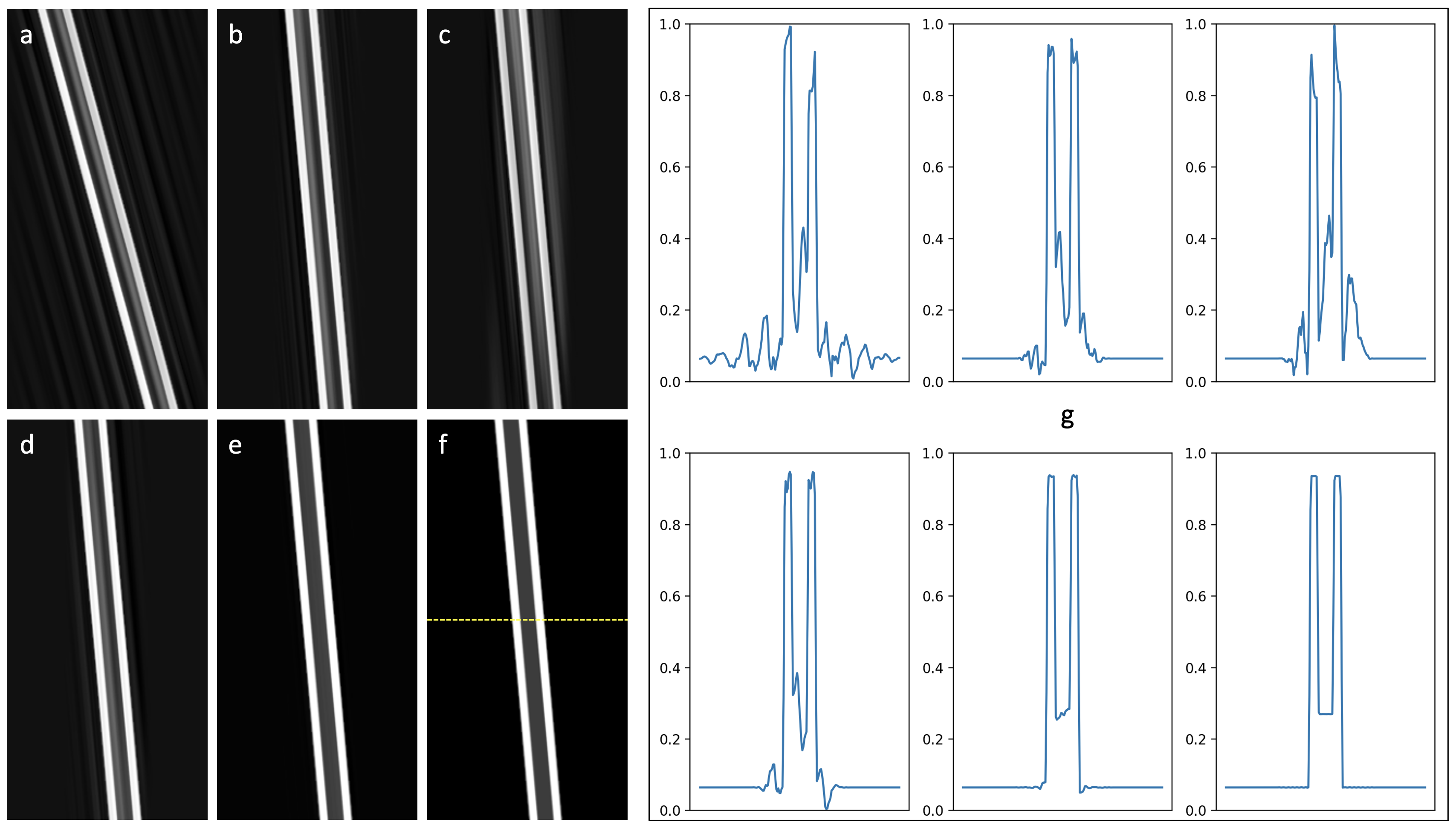
Figure 4. Simulated spine images (cropped) for the five scenarios described in Figure 3 and Table 1 (a-e), and a motion-free reference (f). Image profiles through the line in panel (f) are depicted in (g), showing varying amounts of flow artifact in the cord, CSF, and background tissue. The specific images shown were derived from the upper-bound of the NRMSE distributions in Figure 3.
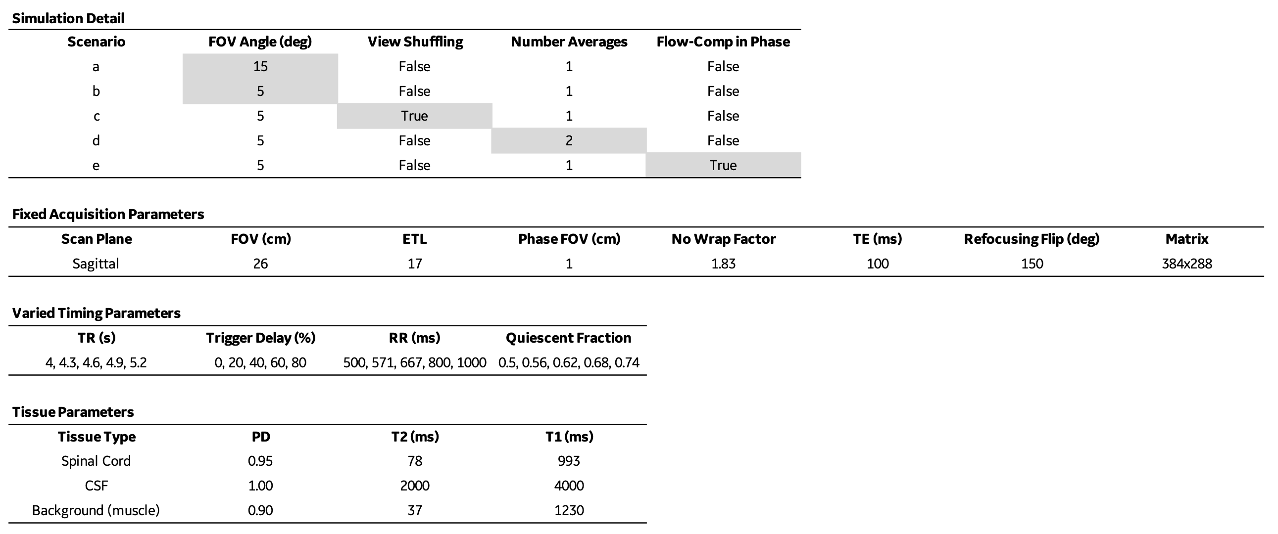
Table 1. Simulation details for the five scenarios depicted in Figures 3 and 4. For each scenario, 625 simulations were performed with the same combination of fixed acquisition parameters and varied timing parameters. All simulations used flow-compensated readout waveforms, and a peak CSF velocity of 10 cm/s. The term "trigger delay" refers to the acquisition start time with respect to the cardiac cycle. The spine phantom tissue phantom parameters referenced in Figure 2 are also listed.
DOI: https://doi.org/10.58530/2023/1556