1486
Influential factors in deep learning classification of clear cell renal carcinoma cancer1Radiology, UT Southwestern Medical Center, Dallas, TX, United States
Synopsis
Keywords: Kidney, Machine Learning/Artificial Intelligence
Deep learning has been successful in predicting tumor malignancy. Clear cell renal carcinoma (ccRCC) diagnosis may help in decision making between active surveillance and definitive intervention. In this study, we investigate the effects of different factors on the performance of deep learning classification of ccRCC using T2w images. We demonstrate that the performance of 15 different CNN models varied substantially. The choice of CNN models, the cropped image size, and the type of inputs greatly altered the performance of ccRCC classification. We achieved the best AUC value of 0.81, which is close to the reported performance of radiologists.
INTRODUCTION:
Clear cell renal cell carcinoma (ccRCC) is the most common and aggressive histologic subtype of renal cell carcinoma (about 70%) 1, 2. Small-renal-masses (SRM, ≤4cm) account for over 50% of renal masses from benign tumors (20%) to aggressive malignancies 1, 3. Active surveillance (AS) is an accepted management strategy for patients with SRMs and even larger localized tumors (4 cm<T1b< 7cm) 4. Identification of ccRCC can help in deciding between AS and definitive intervention 5. A convolutional neural network (CNN) model (Resnet50) was reported for distinguishing benign renal masses from malignant renal tumors 6. Recently, researchers have shown that the squeeze-excitation (SE) module and additional fully-connected (FC) layers can further improve the performance in prediction of vessel invasion in cervical cancer7. In this study, we investigated the performance of different deep learning models for the diagnosis of ccRCC using T2w images.METHODS:
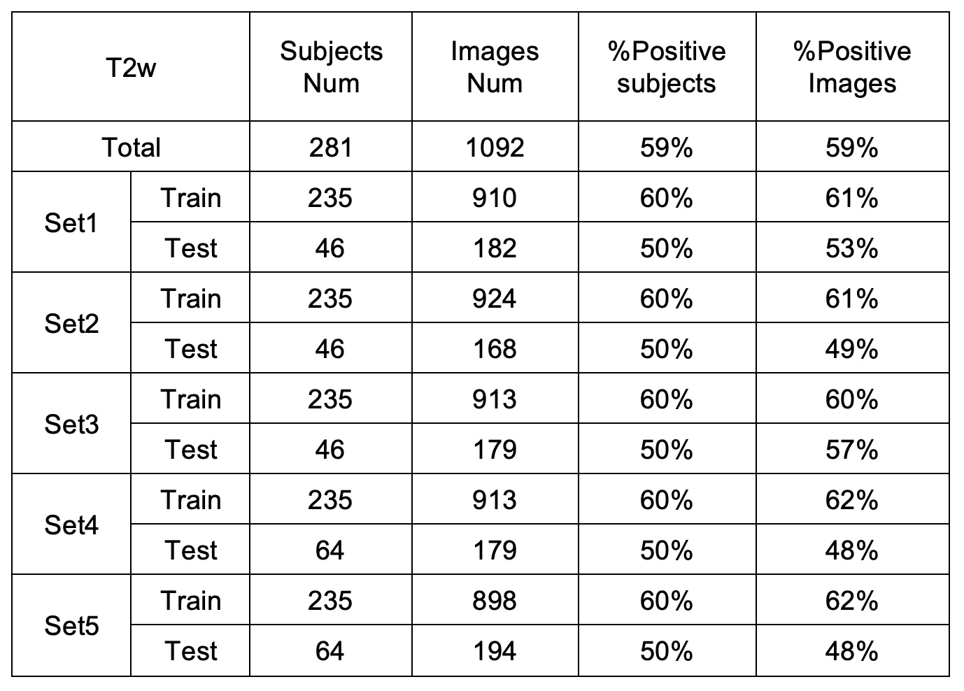
This retrospective study included a total of 281 subjects who under-went surgical resection of a renal mass and had presurgical MR images available for analysis. Coronal T2w single-shot-fast-spin-echo images were acquired on different scanners. Subjects with one tumor and tumor size less than 7 cm were included in this study. Tumor masks were drawn by imaging analysis specialists.First, fifteen CNN models were trained to identify ccRCC. All the CNN models were from or based on the models in the TIMM model library (Pytorch). There were three CNN model architectures (Model1-3) and three different inputs: 1. cropped images only; 2. images and tumor masks; 3. images and Gaussian weight (Gweight) maps (centered at the center of mask with a sigma of 4) as shown in Fig. 1. Second, the effects of different inputs were investigated using two architectures (Model1 and Model3 in Fig.1) based on SEresnet50 model. Finally, the effects of different cropped image sizes were investigated using these two models. Five-fold-cross-validation was used to estimate the performance of each model. A total of 1092 images including a single tumor were selected for training and testing. The images were divided into training (58%), validation (15%), and testing (27%) sets. The three datasets were separated based on subjects instead of slices to prevent the data leaking. The detailed information of different datasets is summarized in Table 1. The preprocessing steps included N4bias-field correction, cropping, and z-score normalization. The data augmentation steps were randomly implemented in every epoch including 2D rotation (-10°~10°), left-right flip, up-down flip, adding gaussian noise, etc. The total number of epochs was 300. Batch size was 100 in most cases and 50 in those cases when the GPU memory requirement exceeded the GPU memory limit.
ROC analysis was performed to calculate area-under-curve (AUC) for each model. Slice-based metrics were first estimated based on the prediction of ccRCC for each slice. Furthermore, subject-based metrics were assessed based on the slice results. The averaged results of all five datasets derived from the cross-validation were computed and reported in this study.
RESULTS:
Figure 2. shows the summary of averaged AUCs for all fifteen CNN models using a cropped T2w image and a Gweight map as inputs. AUCs for all models varied largely from 0.574 to 0.787. The two models based on SEresnet50 achieved the best performance with AUC values of 0.783 and 0.787.Figure 3. shows the results of averaged AUCs using three different inputs and two different models (SEresnet50 and Model3 “SEresnet50”). The mask and the Gaussian weight improved the performance substantially in comparison with those using the cropped image only for both models.
Figure 4. shows the results of averaged AUCs using five different cropped size and two different models (SEresnet50 and Model3 “SEresnet50”). The size varied from 100 to 300 pixels (or 5cm to 15 cm). The AUCs for models using the smaller cropped size were larger than for those using the larger size.
DISCUSSION / CONCLUSION:
The SE module improved the performance from 0.675 to 0.783 for resnet50 (Fig. 2). Although it has been reported that the SE module and additional FC layers can further improve the performance of the model7, the SE module did not improve the performance of the resnet18 model. The additional FC layers didn’t provide robust improvement for any of the models in this study. For the Model3 (Fig. 3), AUCs using Gweight was larger than ones using the mask (0.776 vs. 0.731), which indicates that the mask annotation may not be necessary, and the center points may play the same role as the masks for the identification of ccRCC. Model3 with an image size of 150 (Fig. 4) achieved the best AUC of 0.807, which exceeded the previously reported AUC of 0.71 for differentiation between benign and malignant renal masses using T2w images 6. Although close to the human performance, AUC of 0.807 is still lower than the reported AUC range (0.82-0.92) for diagnosis of ccRCC by radiologists8. In conclusion, we demonstrate that the selected optimized CNN models have a potential to facilitate the identification of ccRCC using T2w images. Future work will investigate whether the performance of these selected models can be further improved by combining other MR images with different contrast.Acknowledgements
This project is supported by NIH grants R01CA154475, U01CA207091, and P50CA196516. We thank Lauren Hinojosa and Ayobami Odu for image annotation.
References
1. Weikert, S. and B. Ljungberg, Contemporary epidemiology of renal cell carcinoma: perspectives of primary prevention. World J Urol, 2010. 28(3): p. 247-52.
2. Campbell, S., et al., Renal Mass and Localized Renal Cancer: AUA Guideline. J Urol, 2017. 198(3): p. 520-529.
3. Frank, I., et al., Solid renal tumors: an analysis of pathological features related to tumor size. J Urol, 2003. 170(6 Pt 1): p. 2217-20.
4. Sebastia, C., et al., Active surveillance of small renal masses. Insights Imaging, 2020. 11(1): p. 63.
5. Johnson, B.A., et al., Diagnostic performance of prospectively assigned clear cell Likelihood scores (ccLS) in small renal masses at multiparametric magnetic resonance imaging. Urol Oncol, 2019. 37(12): p. 941-946.
6. Xi, I.L., et al., Deep Learning to Distinguish Benign from Malignant Renal Lesions Based on Routine MR Imaging. Clin Cancer Res, 2020. 26(8): p. 1944-1952.
7. Jiang, X., et al., MRI Based Radiomics Approach With Deep Learning for Prediction of Vessel Invasion in Early-Stage Cervical Cancer. IEEE/ACM Trans Comput Biol Bioinform, 2021. 18(3): p. 995-1002.
8. Canvasser, N.E., et al., Diagnostic Accuracy of Multiparametric Magnetic Resonance Imaging to Identify Clear Cell Renal Cell Carcinoma in cT1a Renal Masses. J Urol, 2017. 198(4): p. 780-786.
Figures
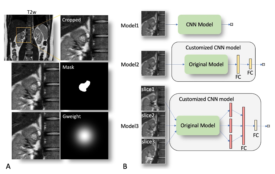
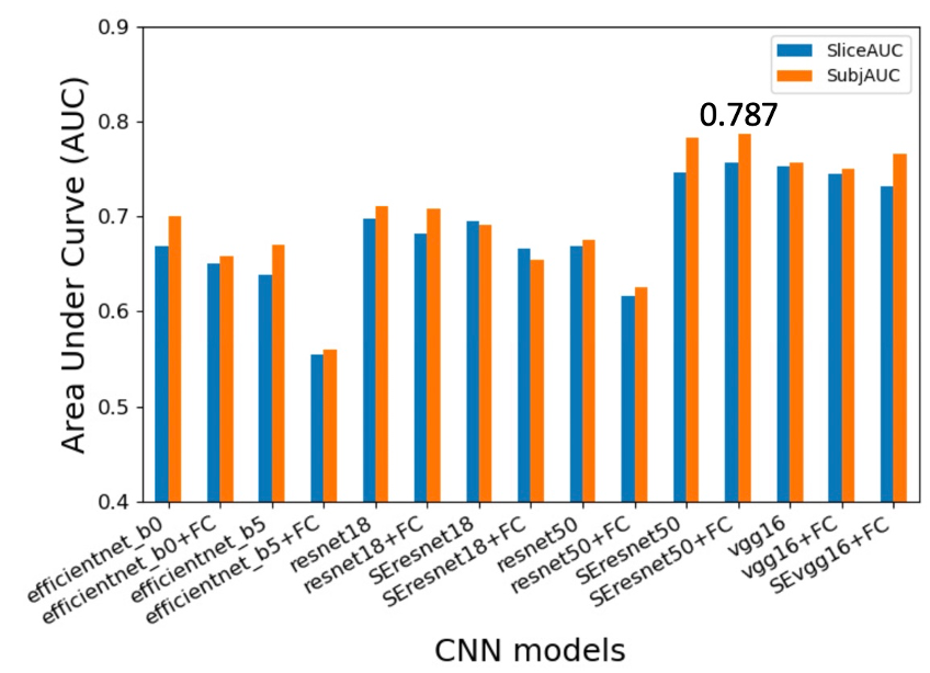
Figure 2. Summary of prediction results using different CNN models with a single T2w image and a Gaussian weight (Gweight) as inputs. Area under curve (AUC) for slices and subjects were plotted for different models. The prefixed “SE” represents the model including the squeeze and excitation attention module; The postfixed “FC” represents fully connected layers in Model 2 in Fig. 1. All these results were from the two architectures (Model 1 or 2 in Fig. 1). The SEresnet50 and SEresnet50+FC models achieved the best results with the values of AUC: 0.783 and 0.787, respectively.
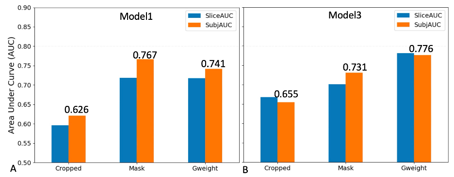
Figure 3. Summary of prediction results using three different inputs for Model1 and Model3 in Fig. 1. A. AUC results using a single slice and Model 1 (SEresnet50); B. AUC results using the three consecutive slices and Model 3, in which the original CNN model is SEresnet50. Cropped represents images only; Mask represents images and mask; Gweight represents images and Gaussian weight. SliceAUC: slice-based AUC; SubjAUC: subject-based AUC.
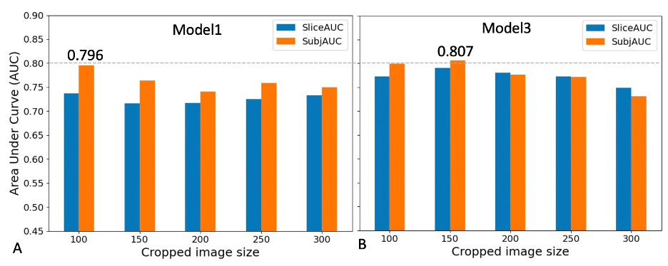
Figure 4. Summary of prediction results for five cropped image sizes using Model1 and Model3 in Fig. 1. A. AUC results using a single slice and Model 1 (SEresnet50); B. AUC results using the three consecutive slices and Model 3, in which the original CNN model is SEresnet50. The inputs were using images and Gaussian weight (Gweight). SliceAUC: slice-based AUC; SubjAUC: subject-based AUC.