1472
Integration of Slice-Based Diagnostic Probabilities Predicted by 2D Deep Learning Using ResNet50 to Yield Lesion-Based Diagnosis in Breast MRI
Yang Zhang1,2, Jiejie Zhou3, Zhongwei Chen3, You-Fan Zhao3, Meihao Wang3, Yan-Lin Liu2, Jeon-Hor Chen2, Ke Nie1, and Min-Ying Su2
1Department of Radiation Oncology, Rutgers-Cancer Institute of New Jersey, New Brunswick, NJ, United States, 2Department of Radiological Sciences, University of California, Irvine, CA, United States, 3Department of Radiology, First Affiliated Hospital of Wenzhou Medical University, Wenzhou, China
1Department of Radiation Oncology, Rutgers-Cancer Institute of New Jersey, New Brunswick, NJ, United States, 2Department of Radiological Sciences, University of California, Irvine, CA, United States, 3Department of Radiology, First Affiliated Hospital of Wenzhou Medical University, Wenzhou, China
Synopsis
Keywords: Cancer, Machine Learning/Artificial Intelligence
A deep learning model using 2D ResNet50 CNN was trained to differentiate a dataset of 103 malignant vs 73 benign breast lesions, then tested in a testing dataset of 53 malignant and 31 benign cases. The 2D slice-based results were used to calculate a probability for each lesion, by using 5 methods: (1) slice-based average, (2) tumor area weighted average, (3) tumor perimeter weighted average, (4) using the probability of the largest tumor slice, (5) using the highest probability among all slices. The results showed using the highest probability to convert from slice-based to lesion-based diagnosis had the best performance.Introduction
Breast MRI is an important clinical imaging modality for the management of breast cancer. The current computer-aided diagnosis (CAD) software is only used for displaying information for the radiologist to give a BI-RADS score indicating the suspicious level of malignancy. Deep learning has been applied to detect and diagnose breast cancer on MRI and shows promising results [1-3]. The output is a malignancy probability. Due to the need for a large dataset for training, deep learning is usually performed using each 2D slice in a lesion as an independent input. A lesion consists of many 2D slices of various sizes and shapes, and a strategy is needed to consider the malignancy probabilities of all slices to give a probability for each lesion, that is, converting from slice-based results to lesion-based diagnosis. So far, few studies have systematically investigated the optimal integration method to convert from 2D slices to a 3D lesion to yield the most accurate results. In order to achieve high sensitivity, the most commonly used method is to assign the highest probability among all slices to that lesion; however, this is at the expense of lowering the specificity. In this study, we applied 2D ResNet50 to train diagnostic models and used 5 different methods to convert the obtained slice-based results to lesion-based diagnostic results. The 5 methods include: (1) the slice-based average to calculate the mean probability from all slices of a lesion, (2) the tumor area weighted average, (3) the tumor perimeter weighted average, (4) the probability of the slice with the largest tumor area, (5) the highest probability among all slices.Methods
This study was conducted using two datasets. The training dataset had a total of 176 cases, including 103 malignant tumors (mean age of patients 55 ± 12) and 73 benign lesions (mean age 42 ± 9). The testing dataset had a total of 84 cases, including 53 malignant tumors (mean age of patients 56 ± 7) and 31 benign lesions (mean age 50 ± 9). The MRI was performed using a GE 3T system. DCE was acquired using 6 frames, one pre-contrast (F1) and 5 post-contrast (F2-F6). Tumors were segmented on contrast-enhanced maps using the fuzzy-C-means (FCM) clustering algorithm [4]. Three heuristic DCE parametric maps were generated according to: the early wash-in signal enhancement (SE) ratio [(F2-F1)/F1]; the maximum SE ratio = [(F3-F1)/F1]; the wash-out slope [(F6-F3)/F3] [2]. The deep learning was performed using 2D ResNet50 convolutional neural networks [2-3], as shown in Figure 1, by using three DCE parametric maps as inputs. For each lesion, the smallest square bounding box containing the entire tumor was generated, and the range of slices for a lesion was determined. The detailed procedures were described in [2]. All 2D slices were used as independent inputs, and the dataset was further augmented by the random affine transformation. The loss function is cross entropy and the optimizer is Adam with a learning rate of 0.001 [7]. ImageNet works as the initial values of the parameters in these models [8]. During training, the 5-fold cross-validation was used to validate the performance, and then the final model was applied to the testing data. The predicted probabilities from all slices of a lesion were processed using the 5 different methods to give a final probability for that lesion. The ROC analysis was performed to evaluate the diagnostic results and for comparison of the 5 methods. The sensitivity, specificity, and accuracy were calculated for each method using the optimal threshold determined from the ROC curve.Results
Three case examples are demonstrated to show the wide range of probabilities from different slices of a lesion. One mass invasive ductal cancer and one non-mass DCIS are shown in Figure 2, and a benign adenosis is shown in Figure 3. The slice thickness was only 1.2 mm so multiple slices were contained in the lesion, and the final probability was calculated using 5 methods. As seen in Figure 2(B), for non-mass DCIS lesions, the probability of some slices can be low, and using the highest probability can correctly diagnose this DCIS and maintain high sensitivity. For the benign adenosis shown in Figure 3, one slice had a probability > 0.5 (0.53), but since the optimal cut-off threshold was 0.54, this case was still correctly diagnosed as benign. The ROC curves are shown in Figure 4. The selected optimal threshold and the diagnostic results in both training and testing datasets are summarized in Table 1. When using the highest malignancy probability among all slices to assign to the lesion, the method had the best performance reaching an AUC of 0.95 in the training set and 0.89 in the testing set. The overall accuracy was 89% in the training set and 83% in the testing set.Conclusion
In this study, we applied 2D ResNet50 deep learning to train diagnostic models for lesions detected on breast MRI, and then used 5 different methods to convert from slice-based prediction results to yield the lesion-based diagnosis. Since the lesion is a 3D structure, it would be best to apply the 3D deep learning network, which has been performed before to analyze brain and achieve satisfactory results [5-6]. However, the 3D CNN architecture requires a high volume of training data to avoid overfitting, and it is also computationally challenging. Thus, the 2D architecture is still widely used, and the conversion from 2D slice-based prediction to 3D lesion-based results is important to yield a clinically interpretable diagnosis. Our results showed that using the highest probability could achieve the best diagnostic AUC and accuracy. Since the threshold was adjusted, this approach also had the highest specificity while maintaining a high sensitivity.Acknowledgements
No acknowledgement found.References
[1] Zhang et al. Automatic Detection and Segmentation of Breast Cancer on MRI Using Mask R-CNN Trained on Non-Fat-Sat Images and Tested on Fat-Sat Images. Acad Radiol. 2022 Jan;29 Suppl 1:S135-S144. doi: 10.1016/j.acra.2020.12.001. [2] Zhou et al. Diagnosis of Benign and Malignant Breast Lesions on DCE-MRI by Using Radiomics and Deep Learning with Consideration of Peri-Tumor Tissue. J Magn Reson Imaging. 2020 Mar;51(3):798-809. doi: 10.1002/jmri.26981 [3] Zhou et al. BI-RADS Reading of Non-Mass Lesions on DCE-MRI and Differential Diagnosis Performed by Radiomics and Deep Learning. Front Oncol. 2021 Nov 1;11:728224. doi: 10.3389/fonc.2021.728224. [4] Nie et al. Quantitative analysis of lesion morphology and texture features for diagnostic prediction in breast MRI. Acad Radiol 2008;15:1513–1525. DOI: 10.1016/j.acra.2008.06.005 [5] Kruthik et al. CBIR system using Capsule Networks and 3D CNN for Alzheimer’s disease diagnosis. Informatics Med. 2019, 14, 59–68, DOI:10.1016/j.imu.2018.12.001. [6] Li et al. H-DenseUNet: Hybrid Densely Connected UNet for Liver and Liver Tumor Segmentation from CT Volumes. IEEE Trans. Med. Imaging 2018 DOI: 10.1109/TMI.2018.2845918Figures
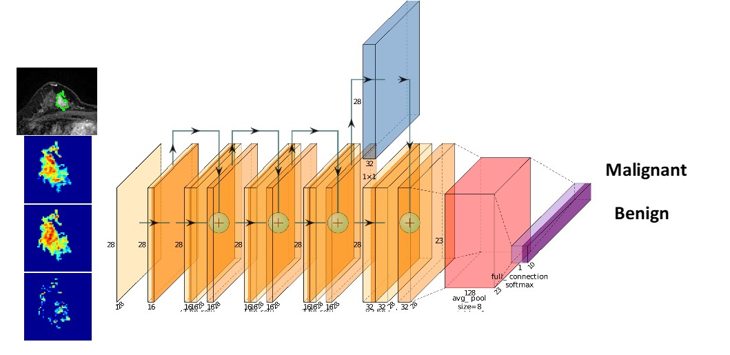
Figure
1:
Architecture
of ResNet50, containing 16 residual blocks. Each residual block begins with one
1 × 1 convolutional layer, followed by one 3 × 3 convolutional layer, and ends
with another 1 × 1 convolutional layer. The output is then added to the input
via a residual connection. The total input channel is 3, using the smallest
bounding box of the three parametric maps. The output is binary, Malignant vs.
Benign, and a malignancy probability is generated for each input slice.
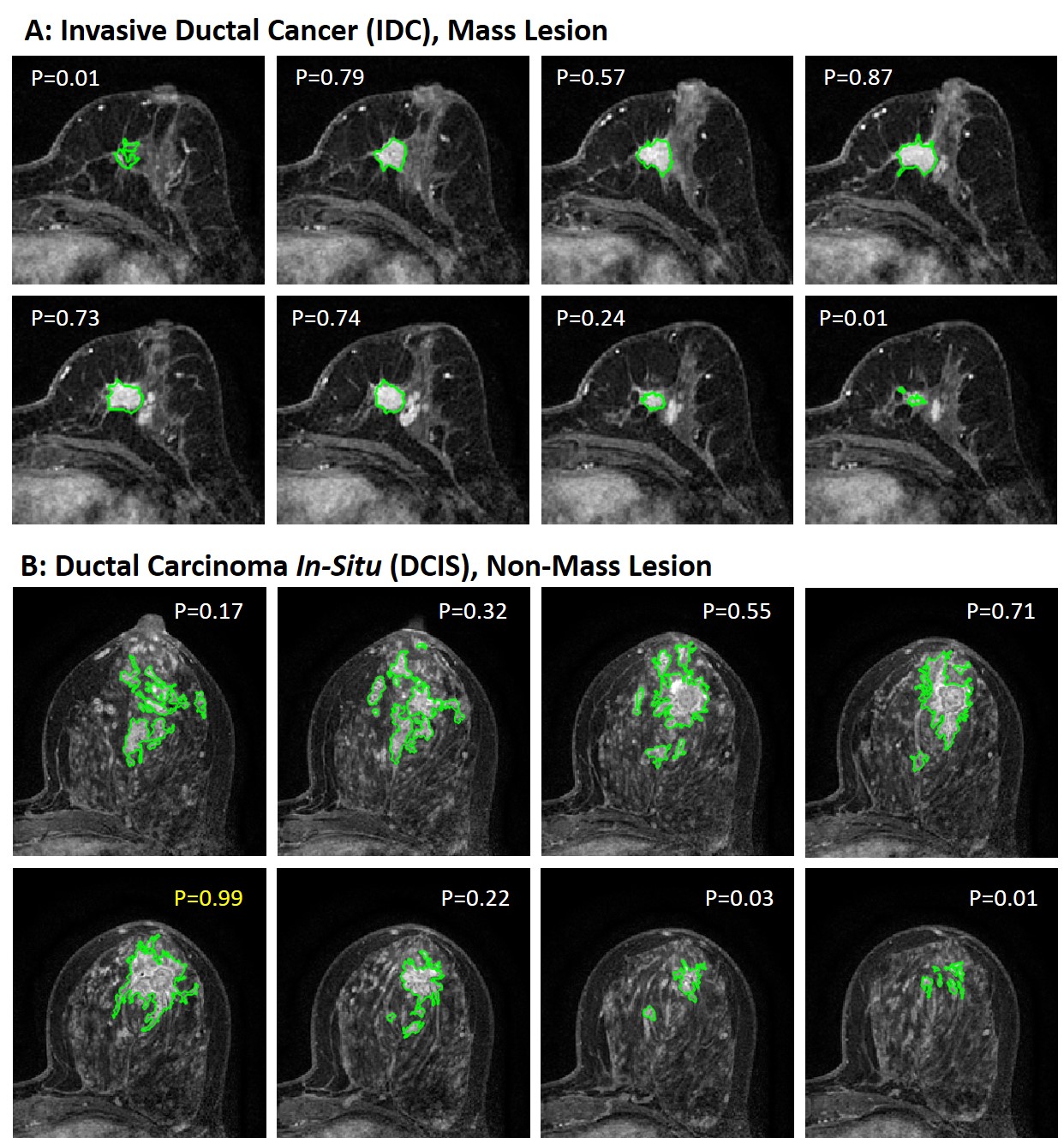
Figure
2: Malignant case examples from (A) A
mass invasive ductal cancer (IDC). The final probability is: (1) mean 0.54; (2)
area-weighted average 0.62; (3) perimeter-weighted average 0.6; (4) the largest
tumor area probability 0.72; and (5) the highest probability 0.87, all correct.
(B) A non-mass ductal carcinoma in-situ (DCIS). The final probability is: (1)
mean 0.38; (2) area-weighted average 0.44; (3) perimeter-weighted average 0.46;
(4) the largest tumor area probability 0.64; and (5) the highest probability
0.99 – the only method yielding a correct diagnosis.
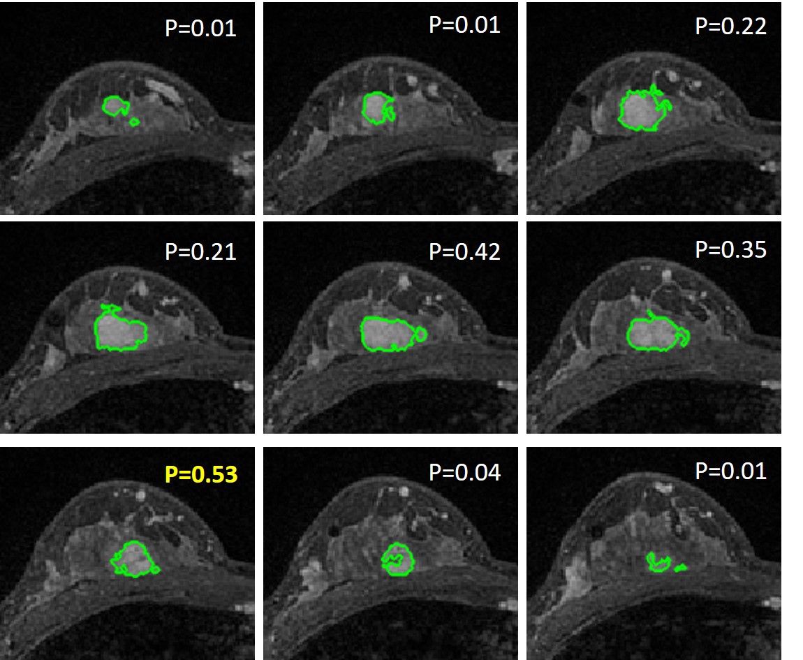
Figure
3:
A benign case example from a
patient diagnosed with histopathologically confirmed adenosis. The predicted
probability for each individual slice is shown. The final probability obtained
using 5 methods are: (1) mean 0.2; (2) area-weighted average 0.31; (3)
perimeter-weighted average 0.29; (4) the largest tumor area probability 0.22;
and (5) the highest probability 0.53. The threshold for Method-5 was 0.54,
so this case is still a true negative using the highest probability.
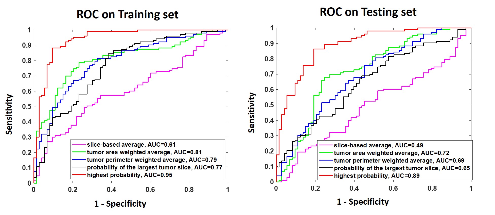
Figure 4: The
ROC curves generated from the predicted lesion-based malignancy probability in
the training and testing dataset, by using the five methods to convert from
slice-based to lesion-based probability.
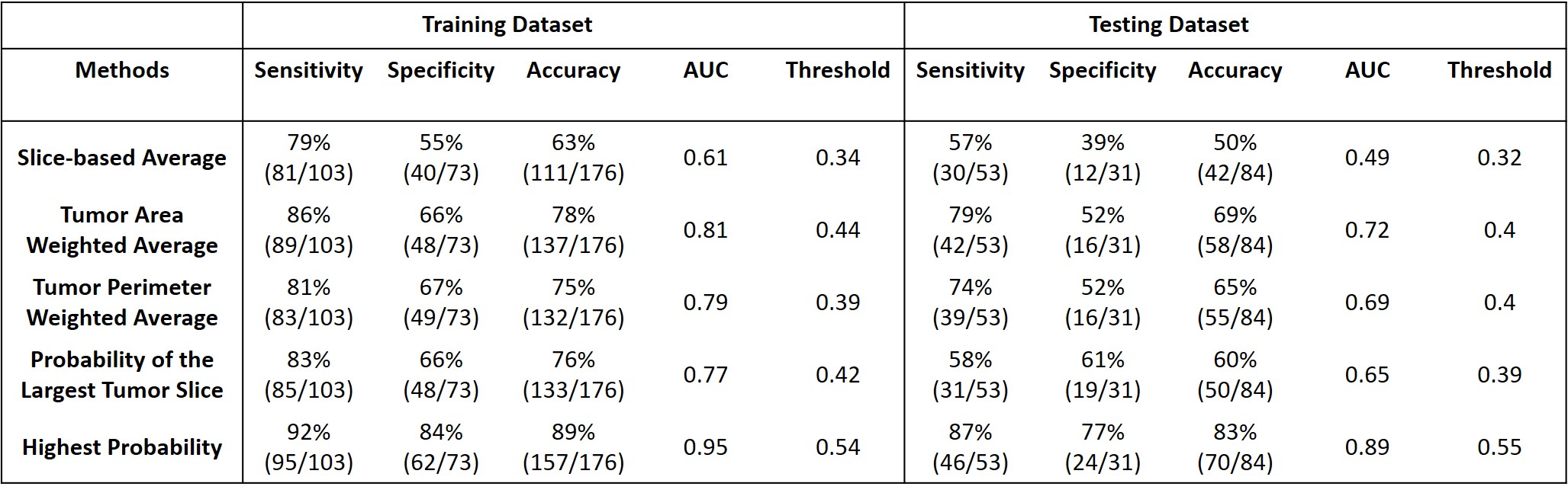
Table 1: The diagnostic sensitivity, specificity,
and overall accuracy obtained by using the optimal thresholds determined from
the ROC curves.
DOI: https://doi.org/10.58530/2023/1472