Synopsis

Keywords: Neurofluids, Neurofluids

It has been suggested that the brain’s waste clearance system involves water exchange between brain tissue and CSF in perivascular spaces, which are part of the subarachnoid space (SAS). In this work, we found CSF T₁ and T₂ in SAS were shorter than corresponding values in the frontal-horns of lateral ventricle, which have minimal exchange. Numerical simulations showed that a higher brain-CSF water exchange rate was associated with lower apparent relaxation time in SAS, providing a potential means to estimate brain-CSF water exchange rate in vivo.

INTRODUCTION

The brain’s waste clearance system is essential for the brain’s homeostasis, and dysfunction of this system may underlie various diseases such as Alzheimer’s disease.¹ Recent studies have suggested that waste clearance involves water exchange between brain tissue and CSF in perivascular spaces, which are part of the subarachnoid space (SAS).^1,2 There has been a growing interest in developing non-invasive MRI techniques to assess the brain-CSF exchange.^3-5 Since brain tissues have much shorter T₁ and T₂ than CSF, the brain-CSF exchange is expected to result in lower apparent relaxation times of CSF in SAS than in regions without active exchange. In this work, we measured CSF T₁ and T₂ in SAS, in reference to corresponding values in the frontal-horns of lateral ventricle, which have minimal exchange. We further performed simulations to link the SAS relaxation time to brain-CSF exchange rate.

METHODS

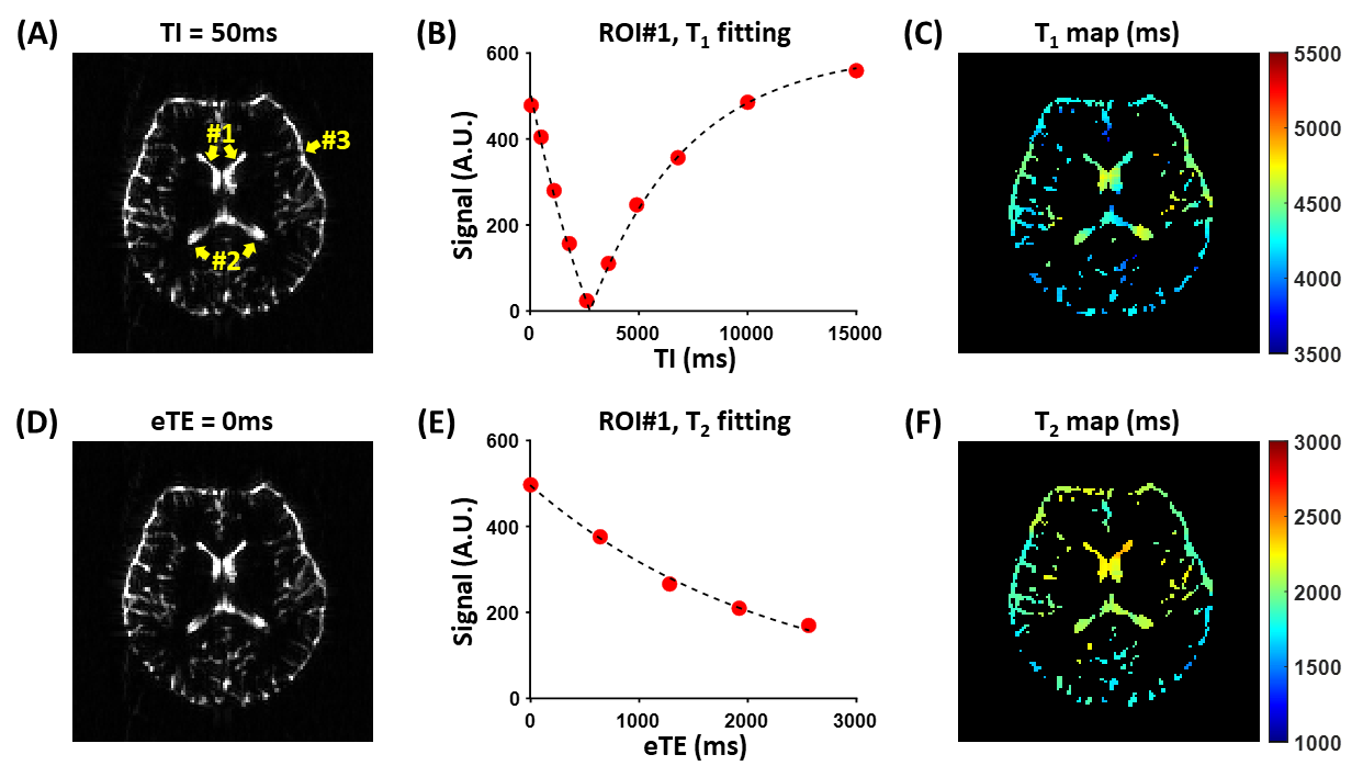
In-vivo Experiments: Seven healthy adults (3F4M, age=24.3±3.1) were scanned on a 3T Siemens Prisma scanner. For CSF-specific (i.e., no tissue or blood contributions) T₁ measurement, we used an adiabatic inversion recovery sequence with spin-echo echo-planar-imaging readout. Ultra-long TE=700ms was used to eliminate partial-volume contamination from brain tissues or blood. 10 TIs of 50,500,1100,1800,2600,3600,4900,6800,10000 and 15000ms were acquired with the following parameters: single-slice of thickness=5mm, field-of-view=218×218mm², resolution=1.7×1.7mm², 2 averages and duration=4.8min.
The sequence for CSF T₂ measurement was similar to that for T₁, except that the inversion recovery module was replaced with T₂-preparation (T₂-prep). Five effective-TEs (eTEs) of T₂-prep: 0,640,1280,1960 and 2560ms were acquired with 2 averages and duration=2min. To examine whether the spacing between refocusing pulses in T₂-prep (τ_CPMG) affected measured T₂, we tested four τ_CPMG: 20,40,80, and 160ms.
To evaluate the reproducibility, each subject underwent three T₁ mapping scans and three T₂ mapping scans with each τ_CPMG.
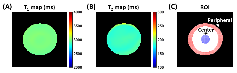
Phantom Experiments: An agarose gel (concentration=0.6%) phantom was scanned using the T₁ and T₂ mapping sequences, to examine whether they had spatially dependent biases in T₁ or T₂ measurement.
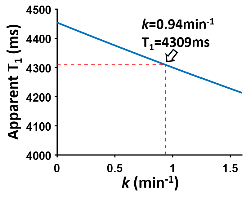
Simulation: To investigate the dependence of apparent SAS T₁ on the brain-CSF exchange rate (k, in unit of min^-1), we simulated the magnetization of CSF spins in SAS using modified Bloch equations:
$$\frac{dM_{z,c1}}{dt}=\frac{M_{0,c1}-M_{z,c1}}{T_{1,c1}}+k({\lambda}M_{z,c2}-M_{z,c1})$$
$$\frac{dM_{z,c2}}{dt}=\frac{M_{0,c2}-M_{z,c2}}{T_{1,c2}}+k(\frac{M_{z,c1}}{\lambda}-M_{z,c2})$$
where the subscripts “c1” and “c2” denote the tissue and SAS compartments, respectively. We assumed tissue T_1,c1=1209ms.⁶ The CSF T_1,c2 used the mean T₁ in the frontal-horns of lateral ventricle measured in in-vivo experiments. λ is the brain/CSF partition coefficient assumed to be 0.8.⁷ The apparent T₁ in SAS was then fitted using the simulated M_z,c2 values for k ranging from 0 to 1.6min^-1.
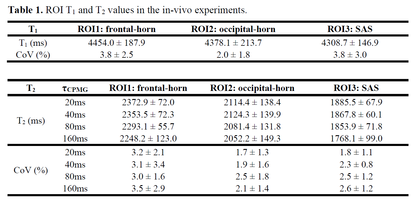
Data Processing: Voxel-wise T₁ and T₂ maps were computed for each scan. For quantitative analyses, T₁ and T₂ values of three regions-of-interest (ROIs) were calculated: ROI1 and ROI2 encompassed the frontal-horns and occipital-horns of lateral ventricle, respectively; ROI3 included all voxels in the SAS (Figure 1A). The coefficient-of-variation (CoV) of the ROI T₁ and T₂ values across the three scans were also computed.
Statistical Analysis: Paired t-tests with Bonferroni correction were used to compare the T₁ values among the three ROIs. For T₂, two-way repeated-measures analysis-of-variance (ANOVA) was used to examine whether the T₂ values differ among ROIs or τ_CPMG values.
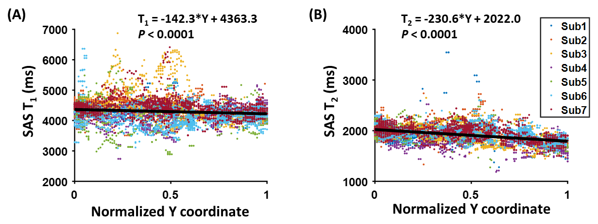
We also evaluated the spatial dependence of SAS T₁ using linear-mixed-effect (LME) analysis. The dependent variable was the T₁ value of a voxel, and the independent variable was the normalized anterior-posterior (Y) coordinate of the voxel (0=anteriormost, 1=posteriormost). This analysis was repeated for SAS T₂ with τ_CPMG=20ms.

RESULTS AND DISCUSSION

In vivo Experiments: Figure 1 shows representative in-vivo data. Table 1 summarizes the ROI T₁ and T₂ values, as well as the CoVs. We found that the frontal-horns of lateral ventricle had higher T₁ than SAS (raw P=0.006, Bonferroni-adjusted P=0.019), while the T₁ in the occipital-horns was not different from the other two ROIs (P>0.2). For T₂, ANOVA revealed significant effects of both ROI (P<0.0001) and τ_CPMG (P<0.0001). The frontal-horns had higher T₂ than the occipital-horns (P=0.03) and SAS (P<0.0001). T₂ values measured with τ_CPMG=20ms were larger than those measured with τ_CPMG=80ms or 160ms (P<0.05).
Moreover, we found that there was a decrease from the frontal SAS to the occipital SAS in both T₁ (P<0.0001, Figure 2A) and T₂ (P<0.0001, Figure 2B).
Phantom Experiments: The phantom T₁ and T₂ maps were relatively uniform (Figure 3). For quantitative comparisons, we computed the T₁ and T₂ values in the center and peripheral regions of the phantom (Figure 3C), and found them to have negligible differences (center T₁=2985.7ms vs. peripheral T₁=2979.5ms; center T₂=188.5ms vs. peripheral T₂=188.8ms). This suggests that the regional differences in T₁ and T₂ observed in in-vivo experiments were not attributable to scanner effects such as B₁ inhomogeneity.
Simulation: As illustrated in Figure 4, a higher exchange rate was associated with a lower apparent T₁ in SAS. The average SAS apparent T₁ of 4308.7ms measured in in-vivo experiments corresponded to an exchange rate of k=0.94min^-1. When dividing the SAS along the anterior-posterior axis, the posterior SAS has a shorter T₁ of 4221.0ms and a higher k=1.55min^-1.

CONCLUSION

We observed that CSF in SAS had lower apparent T₁ and T₂ than the frontal-horns of lateral ventricle, providing a potential means to estimate brain-CSF water exchange rate in vivo.

Acknowledgements

No acknowledgement found.