1421
Rapid mesoscale 3D whole-brain MRF in the Next-Generation 7T brain scanner: challenges and advantages1Department of Radiology, Stanford university, Stanford, CA, United States, 2Department of Electrical Engineering, Stanford university, Stanford, CA, United States, 3Helen Wills Neuroscience Institute, University of California, Berkeley, CA, United States, 4Advanced MRI Technologies, Sebastopol, CA, United States, 5Department of Radiology, University of California, San Francisco, CA, United States, 6San Francisco Veteran Affairs Health Care System, San Francisco, CA, United States, 7Siemens Medical Solutions USA Inc., Berkeley, CA, United States, 8Department of Electrical Engineering and Computer Science, MIT, Cambridge, MA, United States
Synopsis
Keywords: MR Fingerprinting/Synthetic MR, Brain
3D MRF with spiral projection trajectory was implemented on the 7T NexGen scanner to take advantage of its SNR benefit and state-of-the-art gradient system. To achieve high-fidelity and high-efficiency multi-parameter mapping at the mesoscale, novel techniques were developed to overcome several technical challenges in performing this acquisition, including spiral residual gradient compensation, trajectory measurement, water-only excitation RF pulse, B0 correction, B1+ correction and frequency response correction. The proposed technical developments enabled high-quality whole-brain T1, T2, and proton density mapping at 1-mm isotropic resolution in 1 minute, and 560mm isotropic resolution in 4-minutes scan time.Introduction
Ultra-high-filed (UHF) could bring large SNR benefits to MR Fingerprinting(MRF)1 and better gradient system could enable faster sampling2–5. Therefore, the Next-generation(NexGen) 7T scanner6–8 with 96-channel head coil and Gmax=200mT/m and SRmax=900T/m/s presents an excellent platform to enable rapid mesoscale MRF. Nonetheless, there are significant challenges in deploying MRF on this platform, such as severe B0 and B1+ inhomogeneities and gradient imperfections. Building on our previous work9,10 for whole-brain 1-mm 2-minutes MRF at 3T11,12, this work proposed a number of technical innovations for 3D-MRF on UHF, which enables 1-mm MRF scan in 1-minute and 560mm MRF in 4-minutes.Method
Technical challenges and solutions in performing MRF on NexGen 7T scanner:1. Gradient imperfections and eddy currents from fast k-space transversal.
1.1 This can cause the k-space position after rewinder to shift from zero, creating residual gradient area. The amount of residual gradient will vary for TRs as differing spiral interleaves are played out, resulting in imperfect refocusing of the stimulated echoes in FISP-based MRF and thus spatially-varying bias in the T2 estimation.
Solution: Employ Skope13 field probes to measure the residual gradient area per TR and apply a per-TR compensation gradient(Fig1B).
1.2 Gradient trajectory imperfection
Solution: Employ measured spiral trajectories from Skope for reconstruction.
2. B0 inhomogeneity.
2.1 Severe B0 inhomogeneity could cause image blurring and distortion.
Solution: Adopt Multi-frequency-interpolation(MFI)14 into the subspace reconstruction.
2.2 B0 inhomogeneity can cause an RF excitation having spatially-varying flip-angle with areas of severe B0 inhomogeneity experiencing markedly reduced flip angle.
Solution: Calculate the frequency response of RF excitation and introduce a per-voxel flip-angle scaling into the dictionary matching based on B0 inhomogeneity.
2.3 Severe B0 inhomogeneity can spread the fat’s frequency spectrum, making it harder to suppress, causing fat ring artifacts.
Solution: Design water-only SLR RF excitation pulse15 with a broader stop band around the fat frequencies.
3. B1+ inhomogeneity.
Solution: FAs were optimized using Cramér-Rao Bound16 to achieve high accuracy in quantitative estimations across a range of B1+ level and ensure accurate mapping in regions with low B1+. A large range of B1+ scaling [0.01:0.01:1.2] were also incorporated into the dictionary generation.
Sequence: Fig1A shows the MRF sequence diagram using TGAS-SPI trajectory10(Fig1C). Fig1B shows RF and gradients waveforms from one TR, where a non-selective SLR pulse15,17 with duration of 2.86ms, TBW of 3, design parameters ơ1=0.46 and ơ2=0.0001 were used for water-only excitation.
Recon: Fig1D shows the reconstruction pipeline where: i) MFI10,14,18 was incorporated into the subspace reconstruction with demodulation frequency [-500:100:500]Hz. ii) B0 corrected subspace coefficients maps are obtained from this reconstruction. iii) B1+ field map and RF frequency response map jointly generate an FA scaling map for accurate estimation.
Validation: With IRB approval, two healthy volunteers were scanned on a Siemens MAGNETOM Terra Impulse Edition 7T NexGen scanner with a custom 96-channel-Rx abd 16-channel-Tx head coil.
To validate the novel acquisition and reconstruction components, whole-brain 1-mm 3D-MRF data were acquired using low-slew-rate of 100T/m/s (as reference scan with much less gradient error) and high-slew-rate of 600T/m/s within 2min and 1min, respectively. MRF at 560mm isotropic resolution was acquired using 200T/m/s within 4min. FOV is 220x220x220mm3. Additional B0 and B1+ maps were obtained using product sequences with matched FOV at 4-mm resolution.
Results
Fig2A shows varying residual gradient area across TRs using slew-rate of 600T/m/s measured via Skope(left). By adding compensation gradient to create opposing gradient, the residual gradient area is minimized(right) and the T2 estimation improved significantly(red arrows in Fig2C). Fig2B shows the nominal and measured trajectory in a representative TR, and Fig2C(black arrows) shows the improved reconstruction using measured trajectories.Fig3 shows four RF waveforms designed for water-only excitation(Fig3A), along with their frequency responses(Fig3B). Indicated by the red arrows, a strong fat ring artifact is present using 2.94-ms hard pulse, even though it was tuned to have minimal excitation around -1020Hz (the main fat frequency at 7T). That is because the strong B0 inhomogeneity spreads the fat spectrum. The 3-ms Gauss pulse can decrease the fat artifacts(yellow arrows) while the 5.12-ms Gauss and 2.86-ms SLR pulse can further suppress that. The 2.86-ms SLR pulse was finally picked, since it also has a good frequency response across the water frequency band (+/-300Hz) and comparatively shorter duration.
Fig4B shows the T1&T2 maps obtained from reconstructions with i) no correction, ii) B0 correction, ii) B0&B1+ correction, and iv) B0&B1+ &frequency response correction. The B0 correction mitigates image blurring, especially in the frontal lobe with severe B0 inhomogeneity(red arrows). The frequency response correction help further improve the accuracy of T2 estimation(black arrows) in this region.
Fig5A shows the T1&T2 maps at 560mm isotropic resolution, where fine-scale structures and details can be clearly delineated as highlighted in the zoom-in sub-figures. Using the MRF results, clinical contrasts such as MPRAGE(Fig5B), DIR(Fig5C) and 3D MR angiography images(Fig5D) were synthesized. Small-scale structures/features labeled by a neuroradiologist.
Discussion and Conclusion
In this work, we achieved high-fidelity whole-brain MRF at 560mm isotropic resolution in 4min on the 7T NexGen scanner. This was possible through the development and incorporation of a number of novel technical approaches to sequence design, image reconstruction and dictionary matching.Acknowledgements
We acknowledge the help from Dr. Paul Weavers, Dr. Christine Tardif and Sajjad Feizollah on implementing the Skope field probe.
This work was supported in part by NIH research grants: R01-EB020613, R01-EB019437, R01-MH116173, P41EB030006, U01-EB025162, R01MH111444 and 1R44MH129278.
References
1.Ma, D. et al. Magnetic resonance fingerprinting. Nature 495, 187–192 (2013).
2.Akasaka, T., Fujimoto, K., Cloos, M. A. & Okada, T. In-Vivo Evaluation of MR Fingerprinting at 7T Methods : sequence design Methods : image acquisition Methods : post processing & analysis Results & Discussion. 2, 13–16.
3.Cloos, M. A. et al. Multiparametric imaging with heterogeneous radiofrequency fields. Nat. Commun. 7, (2016).
4.Buonincontri, G., Schulte, R. F., Cosottini, M. & Tosetti, M. Spiral MR fingerprinting at 7 T with simultaneous B1 estimation. Magn. Reson. Imaging 41, 1–6 (2017).
5.Koolstra, K., Beenakker, J. W. M., Koken, P., Webb, A. & Börnert, P. Cartesian MR fingerprinting in the eye at 7T using compressed sensing and matrix completion-based reconstructions. Magn. Reson. Med. 81, 2551–2565 (2019).
6.Feinberg, D. A. et al. Design and Development of a Next-Generation 7T human brain scanner with high-performance gradient coil and dense RF arrays. Proc Intl Soc Mag Reson Med 29, 0562 (2021).
7.Gunamony, S. et al. A 16-channel transmit 96-channel receive head coil for NexGen 7T scanner. Ismrm 1–4 (2021).
8.Davids, M. et al. PNS optimization of a high-performance asymmetric gradient coil for head imaging. Ismrm 1–3 (2021).
9.Cao, X. et al. Fast 3D brain MR fingerprinting based on multi-axis spiral projection trajectory. Magn. Reson. Med. 82, 289–301 (2019).
10.Cao, X. et al. Optimized multi‐axis spiral projection MR fingerprinting with subspace reconstruction for rapid whole‐brain high‐isotropic‐resolution quantitative imaging. Magn. Reson. Med. 88, 133–150 (2022).
11.Liang, Z. Spatiotemporal imagingwith partially separable functions. In2007 4th IEEE international symposium on biomedical imaging: from nano to macro 2007 Apr 12 (pp. 988-991).
12.Zhao, B. et al. Improved magnetic resonance fingerprinting reconstruction with low-rank and subspace modeling. Magn. Reson. Med. 79, 933–942 (2018).
13.Dietrich, B. E. et al. A field camera for MR sequence monitoring and system analysis. Magn. Reson. Med. 75, 1831–1840 (2016).
14.Man, L. C., Pauly, J. M. & Macovski, A. Multifrequency interpolation for fast off-resonance correction. Magn. Reson. Med. 37, 785–792 (1997).
15.Norbeck, O. et al. Optimizing 3D EPI for rapid T1-weighted imaging. Magn. Reson. Med. 84, 1441–1455 (2020).
16.Lee, P. K., Watkins, L. E., Anderson, T. I., Buonincontri, G. & Hargreaves, B. A. Flexible and efficient optimization of quantitative sequences using automatic differentiation of Bloch simulations. Magn. Reson. Med. 82, 1438–1451 (2019).
17.Pauly, J., Nishimura, D., Macovski, A. & Roux, P. Le. Parameter Relations for the Shinnar-Le Roux Selective Excitation Pulse Design Algorithm. IEEE Trans. Med. Imaging 10, 53–65 (1991).
18.Ostenson, J., Robison, R. K., Zwart, N. R. & Welch, E. B. Multi-frequency interpolation in spiral magnetic resonance fingerprinting for correction of off-resonance blurring. Magn. Reson. Imaging 41, 63–72 (2017).
Figures
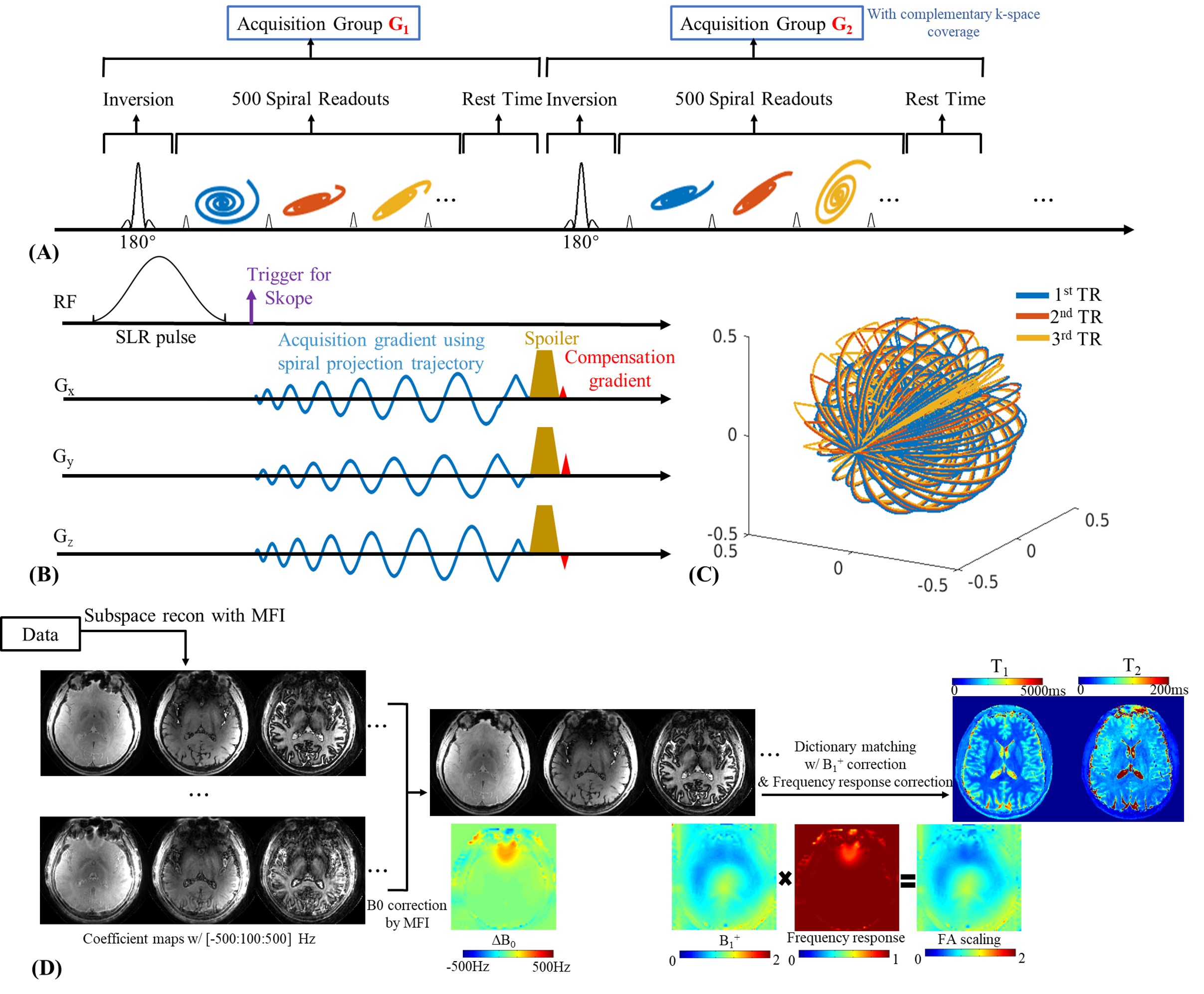
Figure 1.
(A) Sequence framework.
(B) Sequence diagram of one single TR.
(C) The k-space sampling trajectory of 16 groups for the first 3 TRs.
(D) Reconstruction pipeline.
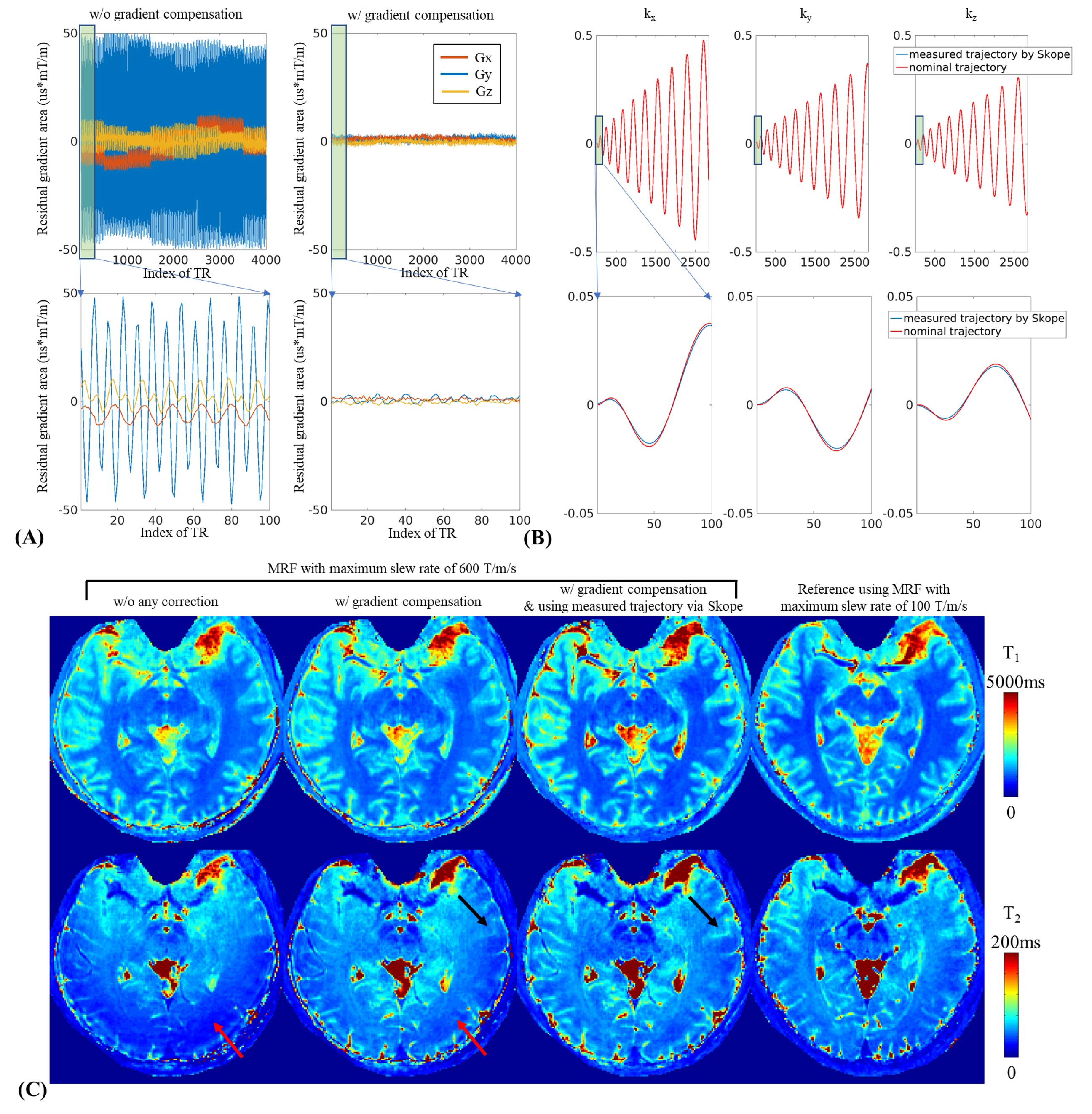
Figure 2.
(A) Residual gradient area after the spiral rewinder for all TRs and the first 100 TRs measured using Skope. With gradient compensation, the residual gradient in all three directions decreased significantly (right).
(B) Measured k-space trajectory using Skope (red lines) and its nominal trajectory (blue lines).
(C) 1-mm T1&T2 maps using rapid 1mm MRF with SRmax=600 T/m/s: i) without any correction, ii) with residual gradient compensation, iii) with residual gradient compensation plus measured trajectory, compare to iv) reference acquisition with SRmax=100 T/m/s.
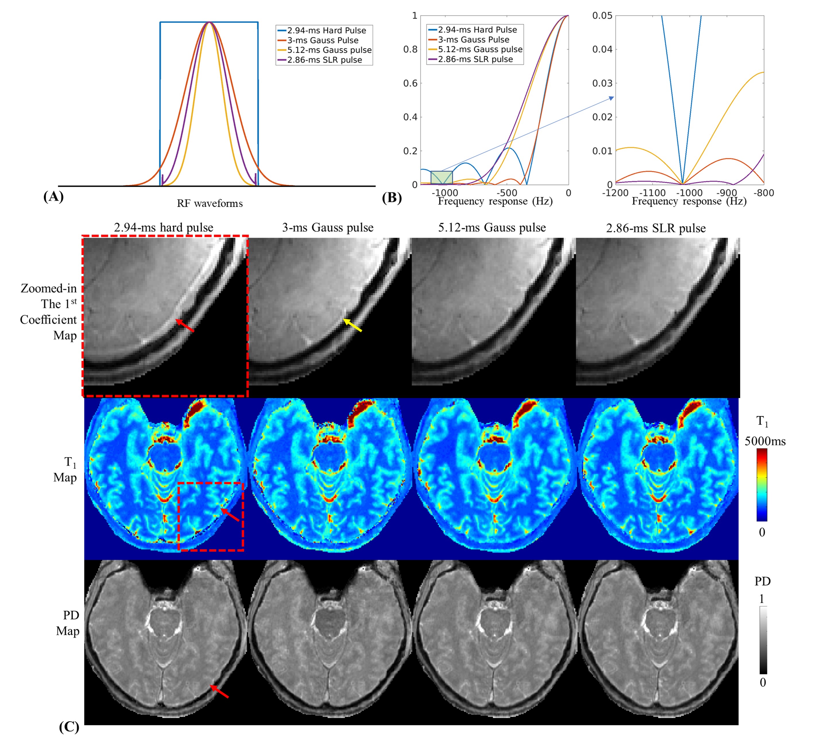
Figure 3.
(A) The waveform of 4 different RF excitation pulses and (B) its corresponding frequency responses.
(C) Zoomed-in the first coefficient maps (top), T1 maps (middle) and proton density maps (bottom) using different RF excitation pulse acquired with 1-min 1-mm MRF.
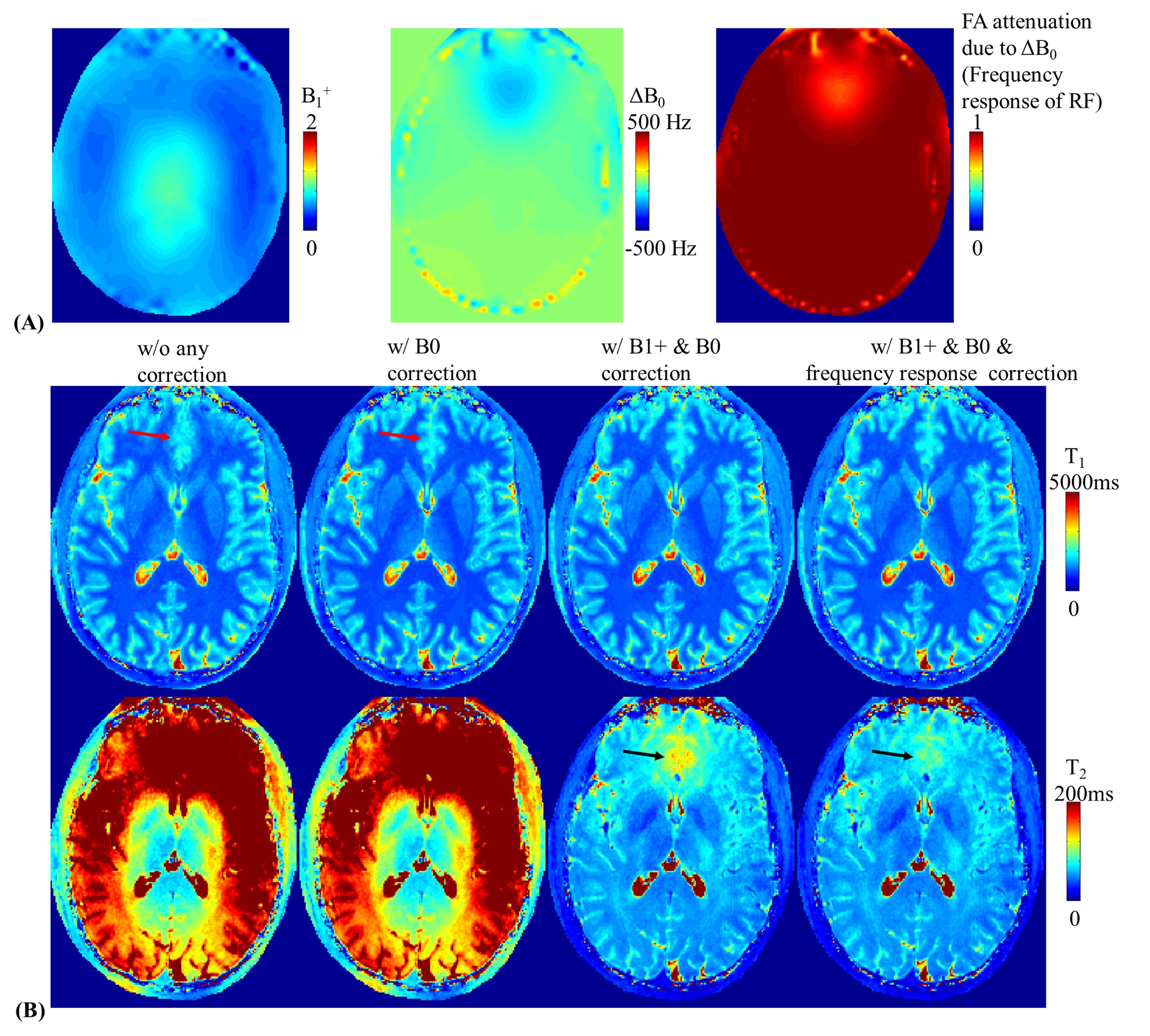
Figure 4.
(A) B1+ map (left), ΔB0 map (middle) and RF pulse’s frequency response map (right).
(B) From left to right: T1 (top) and T2 (bottom) maps without any correction, with B0 correction, with B0 & B1+ correction, and with B0 & B1+ & frequency response correction with 1-min 1-mm MRF.
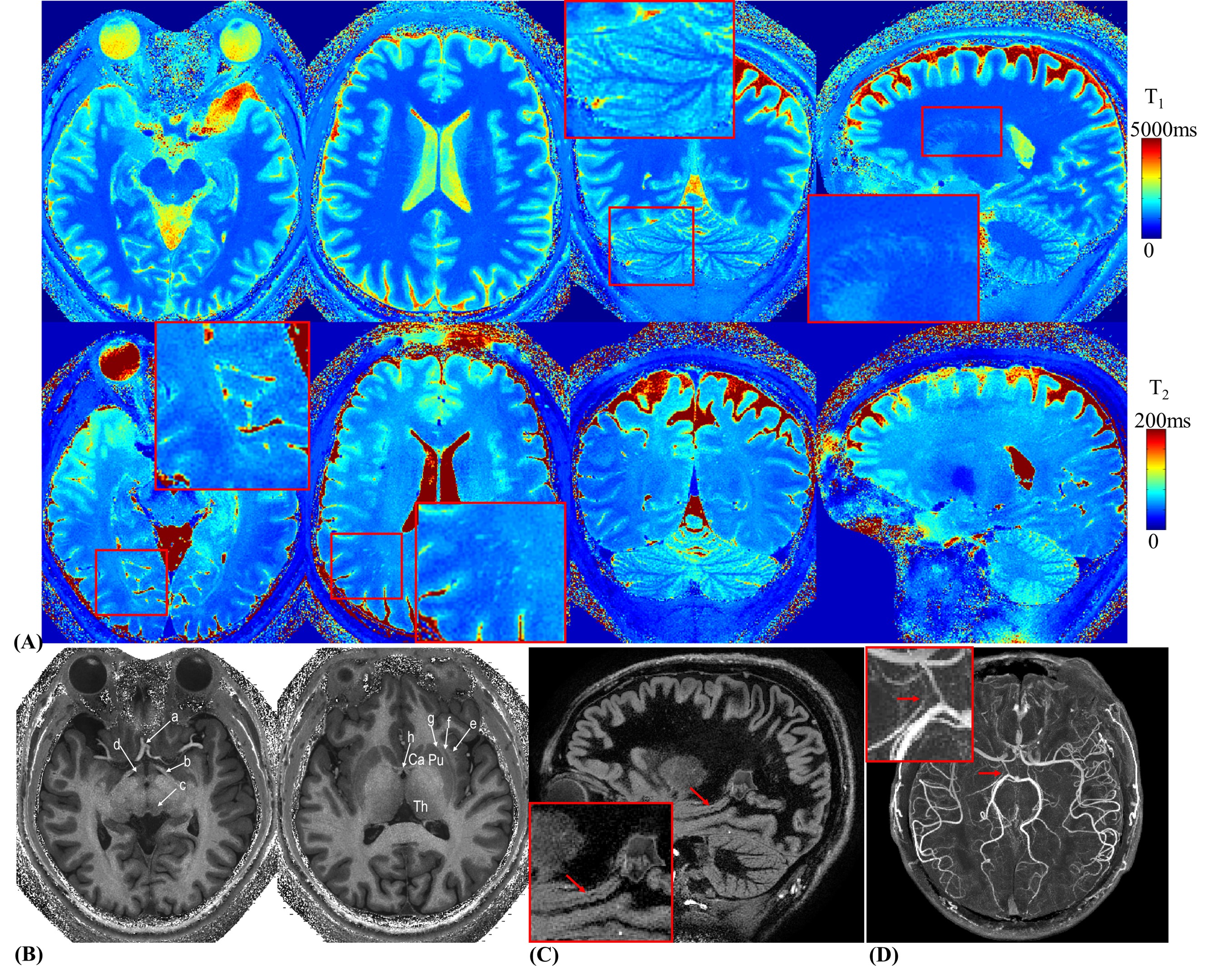
Figure 5.
(A) T1 & T2 with 0.56-mm isotropic resolution obtained in 4min.
(B) Synthesized MPRAGE images using MRF results. Labels: a) anterior communicating artery, b) optic tract, c) superior colliculus, d) hypothalamus, e) extreme capsule, f) claustrum, g) external capsule, h) anterior commissure, Caudate (Ca), putamen (Pu), and thalamus (Th).
(C) Synthesized DIR (double inversion recovery) image using MRF results. Red arrows: the medial occipitotemporal gyrus.
(D) Synthesized 3D MR angiography map using MRF results. Red arrows: the posterior communicating artery.