1391
Improved Visualization of the Medial Medullary Lamina with Phase Prior Reconstruction in Quantitative Susceptibility Mapping
Alexandra Grace Roberts1,2, Ilhami Kovanlikaya2, Brian Koppel3, Pascal Spincemaille2, Thanh Nguyen2, and Yi Wang1,2
1Electrical Engineering, Cornell University, Ithaca, NY, United States, 2Radiology, Weill Cornell Medicine, New York, NY, United States, 3Radiology, Mount Sinai Hospital, New York, NY, United States
1Electrical Engineering, Cornell University, Ithaca, NY, United States, 2Radiology, Weill Cornell Medicine, New York, NY, United States, 3Radiology, Mount Sinai Hospital, New York, NY, United States
Synopsis
Keywords: Parkinson's Disease, Brain
Morphology Enabled Dipole Inversion (MEDI) is an iterative reconstruction algorithm for Quantitative Susceptibility Mapping (QSM) that is effective in suppressing artifacts by exploiting the magnitude image as a morphological prior. Use of a phase prior such as the local field to determine the $$$L_1$$$ regularization term results in improved visualization of the medial medullary lamina as measured by the contrast-to-noise ratio and was preferred by a radiologist over the magnitude prior in each case.Introduction
Quantitative Susceptibility Mapping (QSM) is an MRI contrast mapping the magnetic susceptibility of tissue in vivo from gradient echo measurements. The inverse problem in QSM is ill-posed requiring the use of regularization. Bayesian inference approaches such as Morphology Enabled Dipole Inversion (MEDI) use an edge-weighted gradient under an norm to penalize the streaking and shadowing artifacts arising from dipole-incompatible sources (such as noise) in the phase of the gradient echo data [1], [2], [3]. This is achieved by computing the gradient of the morphological prior and penalizing edges in the reconstruction outside of this gradient. Reduced contrast in the magnitude image can lead to smoothing of fine structures [4] such as the medial medullary lamina (MML), portions of which derive from nerve fibers of the striatum [5]. MLL can be used to define the globus pallidus internus (GPi) which is targeted for deep brain stimulation in the treatment of Parkinson’s disease [6]. The use of a phase-based prior (the local field) is compared to the conventional magnitude prior for the visualization of the medial medullary lamina using the metrics of contrast-to-noise ratio (CNR) and radiologist preference.Theory
The cost function in MEDI+0 [7] is: $$\chi^*(r)=\mathrm{argmin}_{\chi}(‖w(e^{ib}-e^{id*\chi} )‖_2^2+λ_1‖M_M \nabla\chi‖_1+λ_2‖M_{CSF} (χ-\bar{\chi}_{CSF})‖_2^2) \tag{1}$$ where $$$b$$$ is the relative difference field, $$$d$$$ the dipole kernel, $$$\chi$$$ the susceptibility, $$$w$$$ the noise weighting matrix, $$$M_M$$$ morphological weighting matrix, $$$\nabla$$$ the gradient, $$$M_{CSF}$$$ is the CSF mask and $$$\bar{\chi}$$$ the mean susceptibility within such mask. The morphological weighting matrix $$$M_M$$$, or edge mask, is typically acquired by thresholding ($$$T$$$) the gradient of the magnitude image, $$$M_M=T(\nabla|S_0|)$$$ . The relative difference field, or local field $$$b$$$, here called a “phase prior” is defined as $$$M_P=T(\nabla|b|)$$$ and replaces $$$M_M$$$ (the magnitude prior) in the cost function to give $$\chi^*(r)=\mathrm{argmin}_{\chi}(‖w(e^{ib}-e^{id*\chi} )‖_2^2+λ_1‖M_P \nabla\chi‖_1+λ_2‖M_{CSF} (χ-\bar{\chi}_{CSF})‖_2^2) \tag{2}$$Methods
Ten patients were scanned at 3T (GE Healthcare) using a 3D multi-echo spoiled gradient echo sequence. Acquisition parameters were FOV = 25.6 cm, partial FOV factor = 0.8, acquisition matrix size = 320 × 320 × 180, flip angle = 15°, slice thickness = 1 mm, TR = 49 ms, number of echoes = 10, first TE = 4.2 ms, echo spacing = 4.9 ms, parallel imaging factor 2, scan time of ~15 minutes. Each QSM was reconstructed using Equation 1 after nonlinear fitting and region-growing phase unwrapping, [8] projection onto dipole fields (PDF) background field removal [9], and a spherical mean value (SMV) [10] kernel of 5 mm. Regularization parameters were $$$\lambda_1=1000$$$, $$$\lambda_2=100$$$ . For each patient, separate QSMs were reconstructed using the gradient of magnitude and phase prior to generate the edge mask . The QSMs were presented to an experienced (more than 20 years) neuroradiologist, who selected the map with superior MML visualization. The QSM with superior MML visualization was then segmented as shown in Figure 2. The CNR at each boundary was calculated using the standard deviation of susceptibility within the head of the caudate nucleus as a noise reference. The boundaries assessed were the external MML boundary (MML-GPe) and the internal MML boundary (MML-GPi) on the left and right side of the brain. Improvements in the CNR were assessed with a Wilcoxon signed rank test.Results
The phase prior QSM reconstructions provided superior MML visualization according to the radiologist. An example comparison is shown in Figure 3. This qualitative finding is consistent with the increased CNR shown in Figure 4. All CNR improvements were found to be significant at $$$\alpha=0.01$$$.Discussion
As noted in [11], QSM and the magnitude image will generate different contrasts due to differences in the underlying signal generation. Spatial variation in coil sensitivity may reduce the local effectiveness of the magnitude prior due to global thresholding. It is speculated that the phase image does not suffer from this effect at adequate signal-to-noise ratio (SNR). In the magnitude image, the signal is generated by the precession of protons in water molecules following radio-frequency (RF) excitation. Additionally, variations in myelin content were identified as the source of phase contrast between cortical gray and white matter [12] and contrast on the MML QSM is thought to be due to the presence of myelin in the nerve fibers [13], which provides diamagnetic susceptibility contributions. Since the phase image reflects the field generated by tissue susceptibility, it is sensitive to iron deposition and myelin content in the components of the globus pallidus and an alternative prior for QSM reconstruction when the MML is of interest.Acknowledgements
No acknowledgement found.References
- J. Liu et al., “Morphology enabled dipole inversion for quantitative susceptibility mapping using structural consistency between the magnitude image and the susceptibility map,” Neuroimage, vol. 59, no. 3, pp. 2560–2568, 2012.
- Y. Kee et al., “Quantitative susceptibility mapping (QSM) algorithms: Mathematical rationale and computational implementations,” IEEE Trans. Biomed. Eng., vol. 64, no. 11, pp. 2531–2545, 2017.
- A. Roberts, P. Spincemaille, T. Nguyen, and Y. Wang, “MEDI-FM: Field Map Error Guided Regularization for Shadow Reduction” International Society of Magnetic Resonance in Medicine, 2022.
- A. Roberts, P. Spincemaille, T. Nguyen, and Y. Wang, “MEDI-d: Downsampled Morphological Priors for Shadow Reduction in Quantitative Susceptibility Mapping,” International Society of Magnetic Resonance in Medicine, 2021.R.
- Nieuwenhuys, J. Voogd, C. Huijzen. The Human Central Nervous System. 4th ed. Leipzig: Steinkopff; 1980.
- P. A. Starr, L. C. Markun, P. S. Larson, M. M. Volz, A. J. Martin, and J. L. Ostrem, “Interventional MRI–guided deep brain stimulation in pediatric dystonia: first experience with the ClearPoint system”, Journal of Neurosurgery: Pediatrics, vol. 14, no. 4, pp. 400–408, 2014.
- Z. Liu, P. Spincemaille, Y. Yao, Y. Zhang, and Y. Wang, “MEDI+0: Morphology enabled dipole inversion with automatic uniform cerebrospinal fluid zero reference for quantitative susceptibility mapping,” Magn. Reson. Med., vol. 79, no. 5, pp. 2795–2803, 2018.
- T. Liu, C. Wisnieff, M. Lou, W. Chen, P. Spincemaille, and Y. Wang, “Nonlinear formulation of the magnetic field to source relationship for robust quantitative susceptibility mapping: Robust QSM With Nonlinear Data Fidelity Constraint,” Magn. Reson. Med., vol. 69, no. 2, pp. 467–476, 2013.
- T. Liu et al., "A novel background field removal method for MRI using projection onto dipole fields (PDF)," NMR in Biomedicine, vol. 24, no. 9, pp. 1129-1136, 2011, DOI: 10.1002/nbm.1670.
- Y. Wen, D. Zhou, T. Liu, P. Spincemaille, and Y. Wang, “An iterative spherical mean value method for background field removal in MRI: Robust Background Field Removal Using iSMV,” Magn. Reson. Med., vol. 72, no. 4, pp. 1065–1071, 2014.
- T. Liu, S. Eskreis-Winkler, A. D. Schweitzer, W. Chen, M. G. Kaplitt, A. J. Tsiouris, and Y. Wang, “Improved Subthalamic Nucleus Depiction with Quantitative Susceptibility Mapping”, Radiology, vol. 269, no. 1, pp. 216–223, 2013.
- C. Langkammer, N. Krebs, W.
Goessler, E. Scheurer, K. Yen, F. Fazekas, et al. NeuroImage 2012 Vol. 59
Issue 2 Pages 1413-1419. Accession Number: 21893208 DOI:
10.1016/j.neuroimage.2011.08.045
- S.
Ide, S. Kakeda, T. Yoneda, J. Moriya, K. Watanabe, A. Ogasawara, K. Futatsuya,
N. Ohnari, T. Sato, Y. Hiai, A. Matsuyama, H. Fujiwara, M. Hisaoka, and Y.
Korogi, “Internal Structures of the Globus Pallidus in Patients with
Parkinson’s Disease: Evaluation with Phase Difference-enhanced Imaging”,
Magnetic Resonance in Medical Sciences, vol. 16, no. 4, pp. 304–310, 2017
Figures
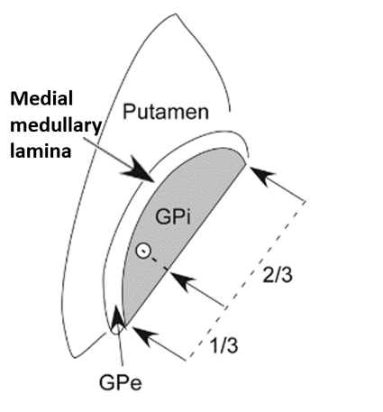
Figure 1. Location of the medial
medullary lamina (MML) relative to the implant target, putamen, globus pallidus
internus (GPi), and globus pallidus externus (GPe). Figure adapted from [5].
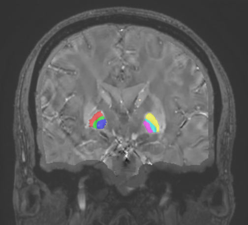
Figure 2. ROI
segmentation for CNR calculation: Left GPe (red), left MML (green), left GPi
(blue), right GPi (pink), right MML (teal), right GPe (yellow), noise reference
(tan).
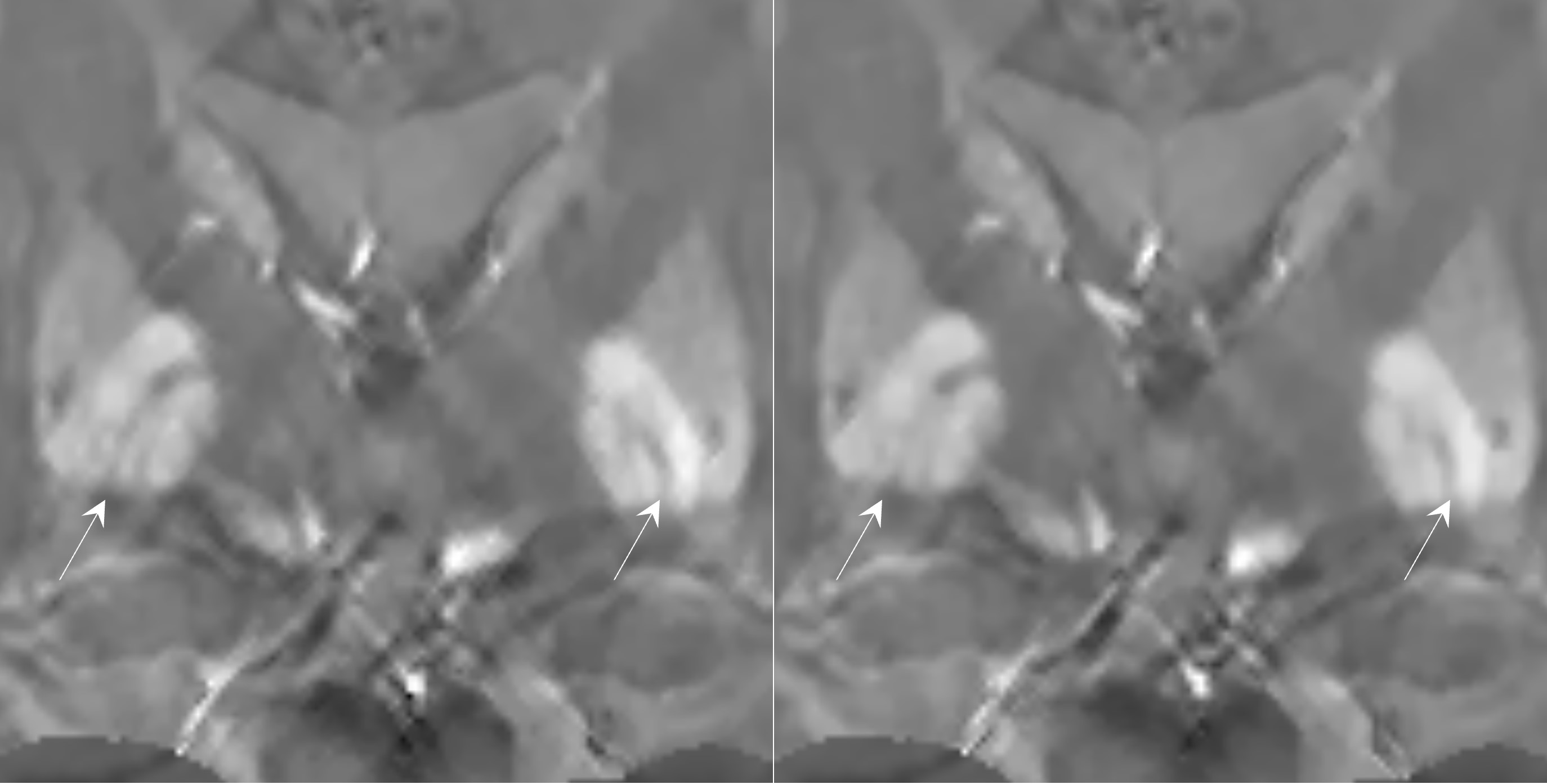
Figure
3. Improved delineation of the MML in the phase prior QSM (left, Equation 2) versus the
magnitude prior QSM (right, Equation 1).
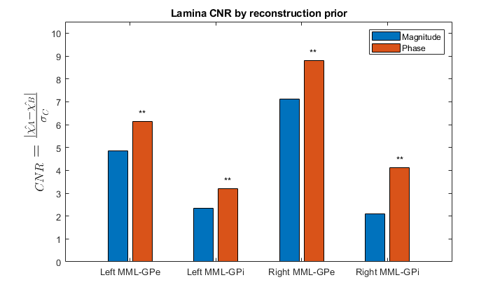
Figure
4. Statistically significant
($$$p=9.77\times10^{-4}$$$) CNR improvements in MML susceptibility.
DOI: https://doi.org/10.58530/2023/1391