1382
Contrast-agnostic segmentation of the spinal cord using deep learning
Sandrine Bédard1, Adrian El Baz1, Uzay Macar1, and Julien Cohen-Adad1,2,3,4
1NeuroPoly Lab, Institute of Biomedical Engineering, Polytechnique Montreal, Montréal, QC, Canada, 2Functional Neuroimaging Unit, CRIUGM, University of Montreal, Montréal, QC, Canada, 3Mila - Quebec AI Institute, Montréal, QC, Canada, 4Centre de recherche du CHU Sainte-Justine, Université de Montréal, Montréal, QC, Canada
1NeuroPoly Lab, Institute of Biomedical Engineering, Polytechnique Montreal, Montréal, QC, Canada, 2Functional Neuroimaging Unit, CRIUGM, University of Montreal, Montréal, QC, Canada, 3Mila - Quebec AI Institute, Montréal, QC, Canada, 4Centre de recherche du CHU Sainte-Justine, Université de Montréal, Montréal, QC, Canada
Synopsis
Keywords: Machine Learning/Artificial Intelligence, Segmentation
Several methods to segment the spinal cord have emerged over the past decade. However, they are dependent on the image contrast, resulting in differences of spinal cord cross-sectional area (CSA), a relevant biomarker in neurodegenerative diseases. We propose a novel method using deep learning that produces the same segmentation regardless of the MRI contrast. Moreover, the segmentation is “soft” (non-binary) and can therefore encode partial volume information. CSA computed with this contrast-agnostic soft segmentation method has lower intra- and inter-subject variability, making it particularly relevant for multi-center studies.Introduction
Spinal cord (SC) segmentation is clinically relevant, notably to compute cross-sectional area (CSA) for the diagnosis and monitoring of neurodegenerative diseases such as multiple sclerosis. Various semi-automatic and automatic methods have emerged over the past decades, but all suffer from the same limitation: SC segmentation depends on the input image contrast. Indeed, MRI acquisition parameters have an impact on the physical appearance of the SC and its boundary with cerebrospinal fluid, resulting in measured CSA that vary across image contrasts 1,2. This phenomenon adds variability in multi-center studies, limiting the sensitivity to detect subtle atrophies. Previous methods 3 proposed different deep learning segmentation models per contrast. While this ensures robust SC segmentation per contrast, it does not ensure that the measured CSA is stable across contrasts. For example, CSA computed on T1w images is lower than that computed on T2w images 1,4. In addition, the use of binary masks is limiting for tissue boundaries that contain a mixture of tissues (partial volume effect). Using soft segmentation 5 could overcome this limitation and help further reduce variability in CSA measures across contrasts. In this study, we propose a contrast-agnostic deep learning model to segment the SC. We show that this approach reduces CSA variability across MRI contrasts.Methods
The overall idea is to train a deep learning segmentation model based on ground truth (GT) segmentations that are averaged across contrasts.Data: We used the Spine Generic Public Database (Multi-Subject) 6 that includes 267 participants and 6 different contrasts: T1w, T2w, T2*w, MT_off, MT_on and DWI.
Data preprocessing: Figure 1 presents an overview of the preprocessing, which was carried on using the Spinal Cord Toolbox (SCT) 7 v5.7. The SC was automatically segmented on all contrasts using sct_deepseg_sc 3. Manual corrections were performed when segmentation was incorrect. Then, for each participant, all contrasts were co-registered to the T2w scan (which has the highest and isotropic resolution). The warping fields were applied to each contrast’s segmentation using trilinear interpolation. Once in the same space, all segmentations were averaged together to produce a single segmentation for this participant. The segmentation is "soft", in that it is encoded in FLOAT with values between 0 and 1. The inverse warping field is then applied to this single segmentation, to bring it back into the native space of each contrast. The pair {contrast, soft segmentation} will later serve as GT for model training.
Training: Deep learning experiments were carried on using the ivadomed framework 8 and used a U-Net network architecture that historically performed well for SC segmentation 5. We investigated various deep learning experimental settings (see Figure 2) to explore: (i) the generalization potential of using one unique model trained with all contrasts (generalist) compared to a set of specific contrast models (one model per contrast); (ii) the benefit of average soft segmentation over the hard segmentation in the context of CSA variability across contrast. The latter will be part of further experiments.
Validation: CSA was computed using sct_process_segmentation 7 across the C2-C3 vertebral levels for: hard GT segmentation, average soft GT segmentation and the testing set prediction mask obtained from the generated models. For each participant, the CSA standard deviation was computed across contrasts in order to evaluate the impact of contrast on CSA measures.
Results
Results of CSA standard deviation for the GT and predicted segmentations are shown in Figure 3. The CSA standard deviation of the average soft segmentation (GT_softmean) is significantly lower (p-value<0.05, paired t-test) than the hard segmentation (GT_binary), confirming that relying on an single soft segmentation across contrasts has the potential to reduce contrast-induced variability. Both deep learning generalist (DL_soft_allcontrast) and specific (DL_soft_percontrast) models produce similar CSA variability, and this variability is significantly lower (p-value<0.05) than the manual hard GT (GT_binary).Discussion
We introduced an image segmentation framework that is minimally sensitive to the input MRI contrast, thereby reducing CSA variability across image contrasts. The output segmentation is ‘soft’, further reducing CSA variability caused by partial volume effects, as previously demonstrated 5. Moreover, we showed that a single deep learning model performs equally well on multiple MRI contrasts when compared to contrast-specific models, which is more convenient, less error-prone, and with a potential for better generalization across out-of-distribution contrasts (ie: not included in training). Further work is needed to validate the performance of the model to other contrasts (MP2RAGE, PSIR, etc.) and pathologies (lesions, cord compression, etc.), and to package the method in SCT 7. We hope the present work will help reduce the required sample sizes in trials when using CSA as a biomarker 4.Acknowledgements
We thank Étienne Bergeron, Olivier Lupien-Morin, Benjamin Carrier and Yassine El Bouchaibi for helping with the manual corrections and labeling, Nicholas Guenther, Alexandru Foias and Mathieu Guay-Paquet for data management with git-annex. We thank Konstantinos Nasiotis and Charley Gros for the insightful discussions.References
1. Cohen-Adad, J. et al. Open-access quantitative MRI data of the spinal cord and reproducibility across participants, sites and manufacturers. Sci Data 8, 251 (2021).2. Kim, G. et al. T1- vs. T2-based MRI measures of spinal cord volume in healthy subjects and patients with multiple sclerosis. BMC Neurol. 15, 124 (2015).
3. Gros, C. et al. Automatic segmentation of the spinal cord and intramedullary multiple sclerosis lesions with convolutional neural networks. Neuroimage 184, 901–915 (2019).
4. Bautin, P. & Cohen-Adad, J. Minimum detectable spinal cord atrophy with automatic segmentation: Investigations using an open-access dataset of healthy participants. Neuroimage Clin 32, 102849 (2021).
5. Gros, C., Lemay, A. & Cohen-Adad, J. SoftSeg: Advantages of soft versus binary training for image segmentation. Med. Image Anal. 71, 102038 (2021).
6. Cohen-Adad, J. et al. Spine Generic Public Database (Multi-Subject). (2020). doi:10.5281/zenodo.4299140.
7. De Leener, B. et al. SCT: Spinal Cord Toolbox, an open-source software for processing spinal cord MRI data. Neuroimage 145, 24–43 (2017).
8. Gros, C. et al. Ivadomed: A medical imaging deep learning toolbox. Journal of Open Source Software 6, 2868 (2021).
Figures
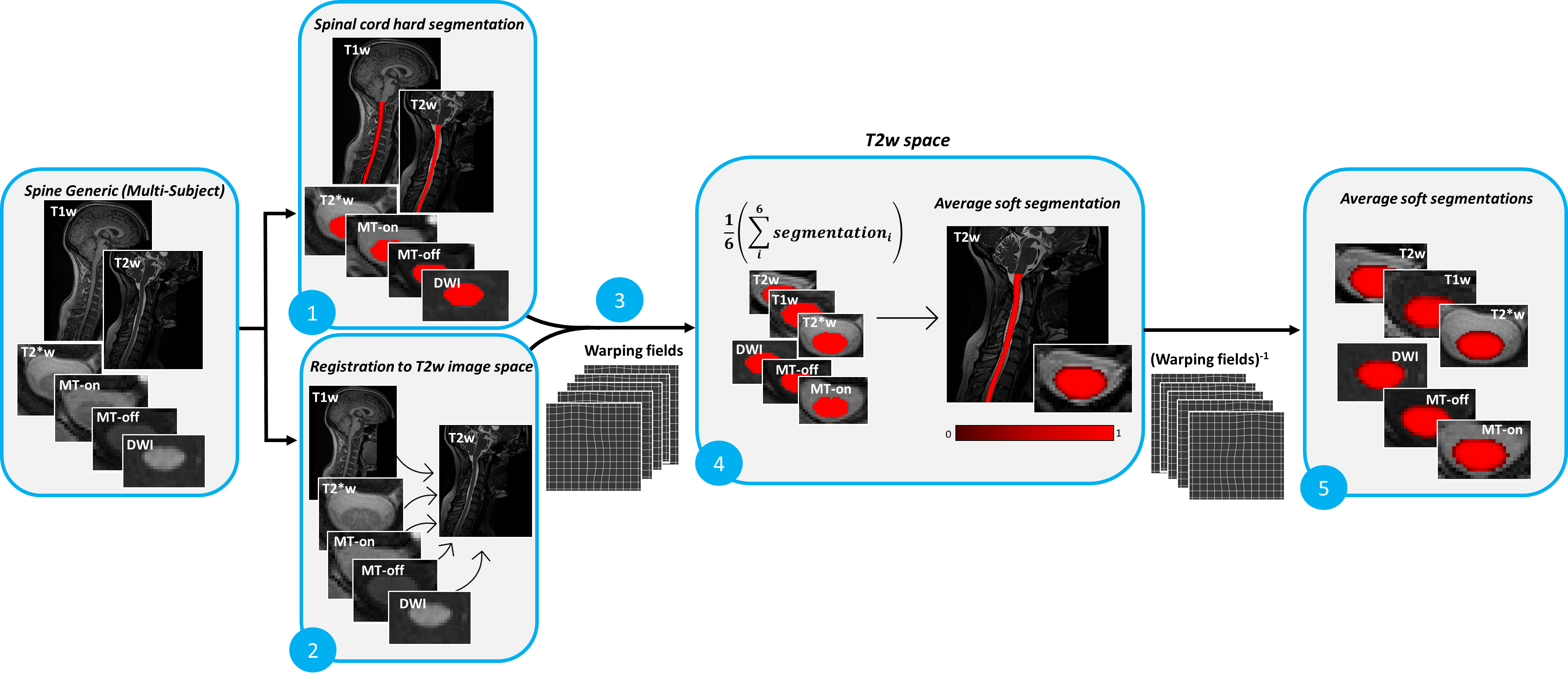
Figure 1. Preprocessing pipeline to generate average soft segmentation GT. (1) Spinal cord was segmented automatically for six contrasts of the Spine Generic Multi-Subject dataset. Manual corrections were applied when errors occurred. (2) All images were registered to the T2w image space. (3) The warping fields were applied to the segmentations. (4) In the T2w space, all segmentations were averaged together to generate one soft segmentation. (5) The inverse warping field was applied to the average soft segmentation and we obtained the soft segmentation in each original image space.
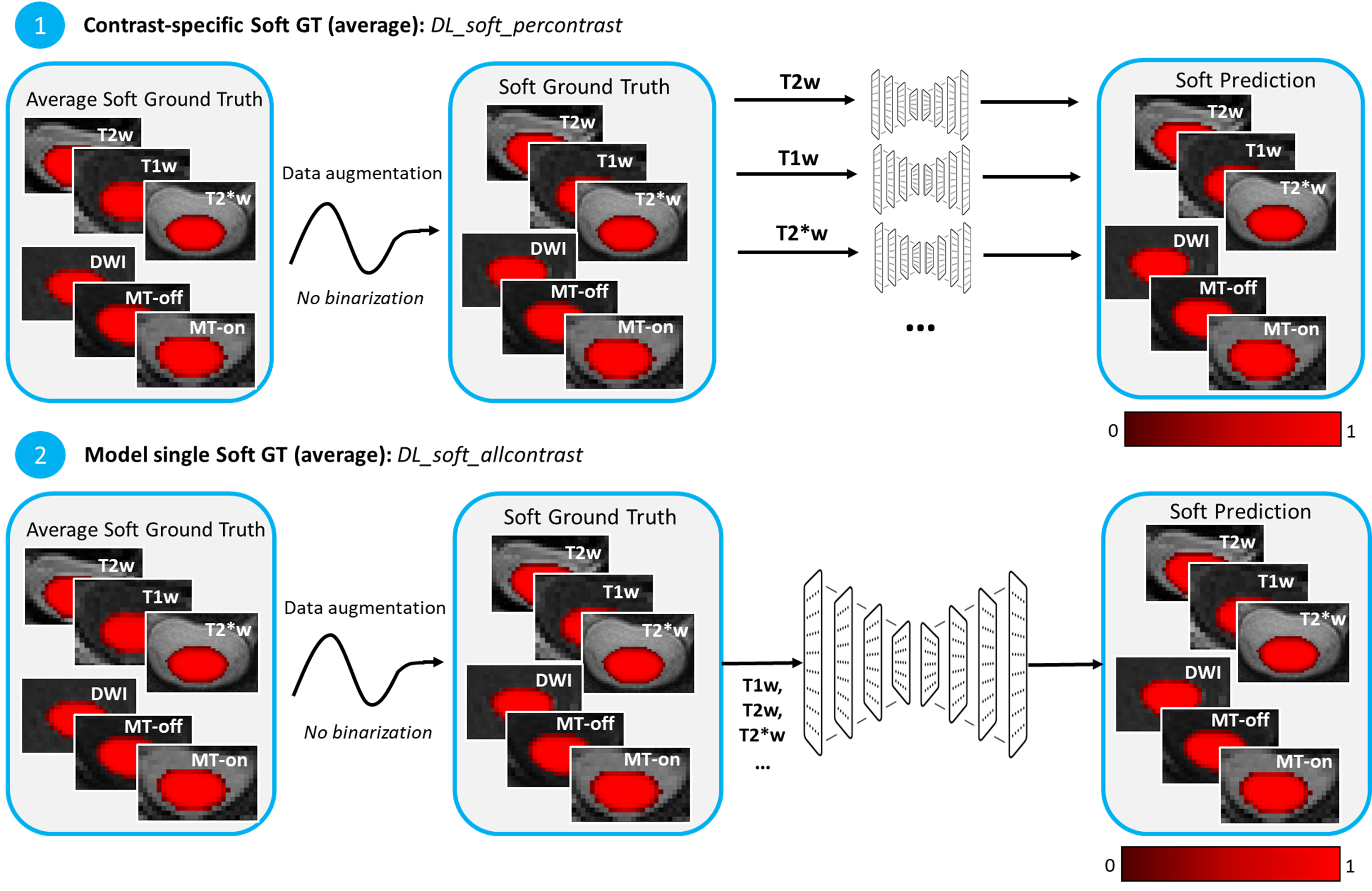
Figure 2. Deep learning experiment settings. (1) DL_soft_percontrast: Average soft ground truth wasn’t binarized after data augmentation; one model per contrast was generated. (2) DL_soft_allcontrast: Average soft ground truth wasn’t binarized after data augmentation; one model for all contrasts was generated.
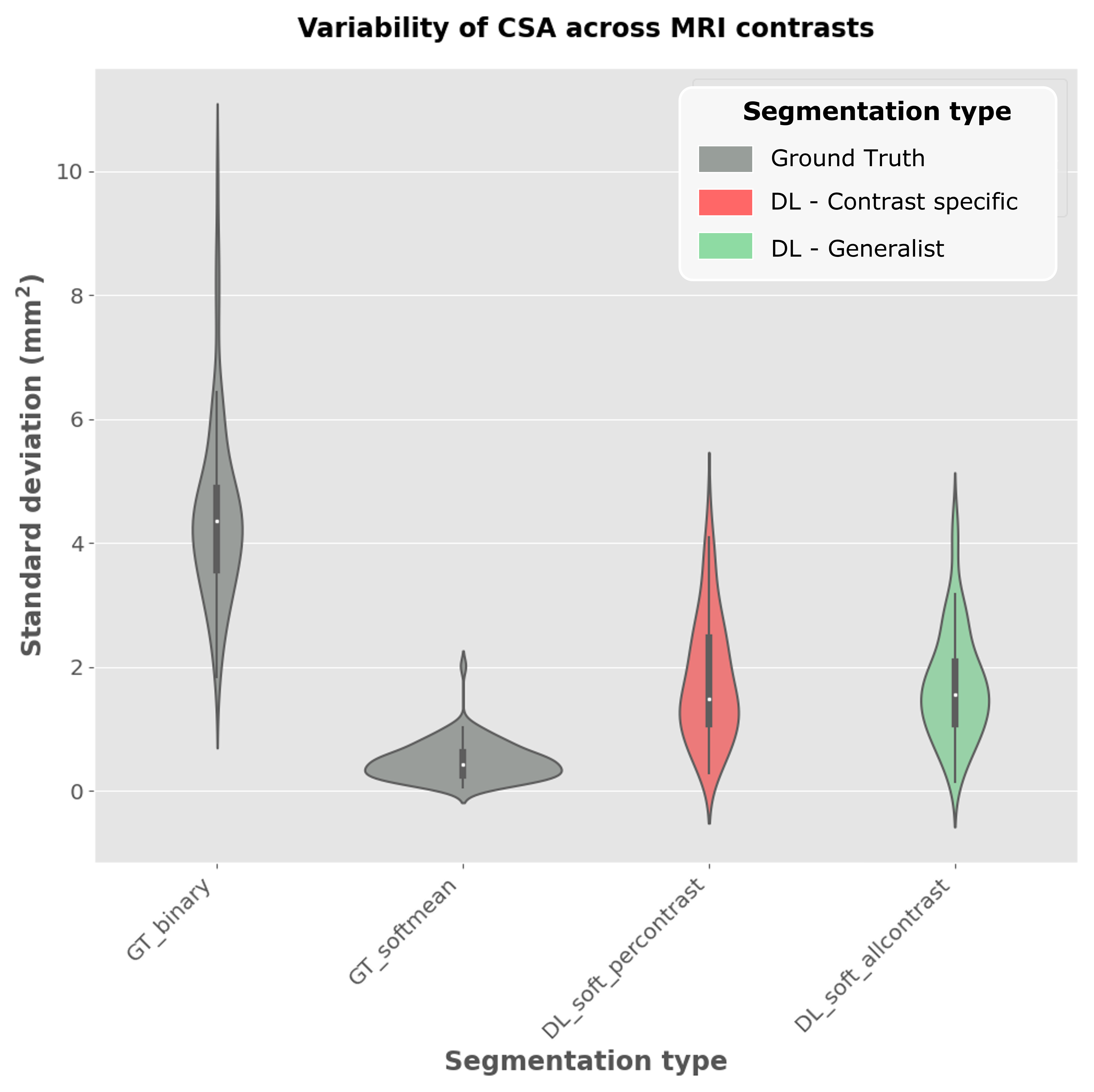
Figure 3. Violin plots of intra-participant CSA standard deviation across all available contrasts. Preliminary results were aggregated for 3 different training seeds. CSA was computed using: hard segmentation ground truth (GT_binary), average soft segmentation ground truth (GT_softmean), “specific” DL segmentation, where the average soft segmentations were used to train one model per contrast (DL_soft_percontrast) and “Generalist” DL segmentation, where the average soft segmentations were used to train one unique model for all contrasts (DL_soft_allcontrast).
DOI: https://doi.org/10.58530/2023/1382