1242
Overcoming system imperfections using end-to-end MR sequence design.
Daniel West1, Felix Glang2, Jonathan Endres3, Moritz Zaiss3, Jo Hajnal1,4, and Shaihan Malik1,4
1Department of Biomedical Engineering, King's College London, London, United Kingdom, 2Magnetic Resonance Center, Max Planck Institute for Biological Cybernetics, Tübingen, Germany, 3Department of Neuroradiology, Universitätsklinik Erlangen, Erlangen, Germany, 4Centre for the Developing Brain, King's College London, London, United Kingdom
1Department of Biomedical Engineering, King's College London, London, United Kingdom, 2Magnetic Resonance Center, Max Planck Institute for Biological Cybernetics, Tübingen, Germany, 3Department of Neuroradiology, Universitätsklinik Erlangen, Erlangen, Germany, 4Centre for the Developing Brain, King's College London, London, United Kingdom
Synopsis
Keywords: System Imperfections: Measurement & Correction, Pulse Sequence Design
MRI systems are usually engineered to give 'ideal' performance, and acquisition methods are generally developed using this assumption. This work proposes an alternative sequence learning framework that includes a model of realistic scanner performance, allowing acquisition sequences to be designed to directly account for system imperfections. In this proof-of-concept demonstration we designed pulse sequences to account for eddy current perturbations with different realistic time constants, while also respecting hardware limits. The flexibility of this approach could be used to design new types of pulse sequence to operate on lower performance, lower cost hardware in future.Introduction
MRI scanners are usually engineered to give close to ideal performance such that acquisition methods can operate under this assumption. Separate strategies are developed to overcome individual imperfections which can lead to an inefficient use of resources; a voltage overhead is required for pre-emphasis, for example. Here we propose a sequence design framework that explicitly accounts for system imperfections and can learn strategies to overcome them.We have built on the recently proposed "MRzero" supervised self-learning pipeline1 that can discover MRI pulse sequences via knowledge of the Bloch equations only. The effectiveness of our approach is shown by optimizing sequences in the presence of eddy currents, with or without applying hardware performance limits.
Theory
Sequences are usually designed by considering a gradient waveform and respecting fixed amplitude and slew rate limits on the gradients themselves. In most scanners, gradient systems are driven under voltage control, often with corrections (e.g. pre-emphasis) as a hidden layer. Thus the designer works with a specified gradient waveform $$$\mathrm{G}(t)$$$ but the gradient amplifier delivers a different hidden voltage waveform $$$\mathrm{V}(t)$$$. Instead we directly formulate the sequence design problem in terms of $$$\mathrm{V}(t)$$$ and connect this to $$$\mathrm{G}(t)$$$ via a physical model. The model could include many effects but here we focus on exponentially decaying eddy currents as in Equation 1:$$[1]\;\mathrm{G}(t)=\beta\left\{\mathrm{V}(t)-\frac{Δ\mathrm{V}}{Δt}\otimes\mathrm{H}(t)\sum_{n}\alpha_n\exp\left(-\frac{t}{\tau_n}\right)\right\}$$
Here $$$\beta$$$ is the 'sensitivity' of the gradient system (mT/m/V), $$$\alpha_n$$$ and $$$\tau_n$$$ are amplitude and time constants for each eddy current term2 and $$$\mathrm{H}(t)$$$ is a unit step function. Physical constraints actually apply to $$$\mathrm{V}(t)$$$ whereas $$$\mathrm{G}(t)$$$ defines the k-space trajectory for imaging, incorporated into forward MR signal simulation within the optimization. The pipeline compared to a more conventional approach is presented in Figure 1.
Methods
Starting from a base sequence with defined initial waveforms $$$\mathrm{V}(t)$$$, the sequence is first simulated assuming perfect system performance (i.e. $$$\mathrm{G}(t)=\beta\mathrm{V}(t)$$$) to determine a 'target' k-space $$$\mathrm{k_T}$$$ and via Bloch simulation, image $$$\mathrm{I_T}$$$. Subsequently, a true forward model is used to predict the actual k-space $$$\mathrm{k_C}$$$ and image $$$\mathrm{I_C}$$$; crucially this image is always reconstructed via iFFT assuming k-space locations $$$\mathrm{k_T}$$$. Optimization of $$$\mathrm{V}(t)$$$ then uses a composite loss function comprising: (i) an image loss term; (ii) a k-distance loss term; (iii) a voltage term; and (iv) a slew rate term. $$$\mathrm{V_{max}}$$$ and $$$\mathrm{S_{max}}$$$ are voltage and slew rate limits respectively and $$$w$$$ are tunable regularization weights.$$[\mathrm{2a}]\;\mathrm{Total\;Loss}=L_{\mathrm{I}}+L_{\mathrm{k}}+L_{\mathrm{V}}+L_{\mathrm{S}}$$
$$[\mathrm{2b}]\;L_{\mathrm{I}}=w_{\mathrm{I}}\left(\sqrt{\sum\left|\left(\mathrm{I_T}-\mathrm{I_C}\right)\right|^2}\right)$$
$$[\mathrm{2c}]\;L_{\mathrm{k}}=w_{\mathrm{k}}\left(\sum\left(\mathrm{k_T}-\mathrm{k_C}\right)^2\right)$$
$$[\mathrm{2d}]\;L_{\mathrm{V}}=w_{\mathrm{V}}\sum\left(\left|\mathrm{V}(t)\right|-\mathrm{V_{max}}\right)\mathrm{H}\left(\left|\mathrm{V}(t)\right|-\mathrm{V_{max}}\right)$$
$$[\mathrm{2e}]\;L_{\mathrm{S}}=w_{\mathrm{S}}\sum\left(\left|\frac{Δ\mathrm{V}}{Δt}\right|-\mathrm{S_{max}}\right)\mathrm{H}\left(\left|\frac{Δ\mathrm{V}}{Δt}\right|-\mathrm{S_{max}}\right)$$
Optimizations used the Adam3 algorithm with an initial learning rate of 0.001.
Throughout, a spoiled gradient echo sequence with FA = 5° and TR = 10ms was used as the starting point. A numerical brain phantom with feasible B0, B1, T1, T2, T2', PD and isotropic diffusion coefficient values was used for signal simulation using a novel phase graph approach4. Time was discretized into steps $$$Δt$$$ = 0.1ms, with the first 2ms of each TR reserved for RF pulses (no gradients) and an acquisition window of 3.2ms (0.5ms after the RF pulse). Images were simulated on a 32x32 grid, and all TR periods were simulated to allow for longer-term eddy currents whose effect persists over multiple periods.
An unconstrained scenario (no hardware limits; $$$w_{\mathrm{V}}=w_{\mathrm{S}}=0$$$) was considered with eddy currents having $$$\tau_n$$$ = 0.5ms or 50ms, and together as a bi-exponential perturbation; $$$\alpha_n$$$ = 0.5 was used for all cases. Constrained optimizations using $$$\beta\mathrm{V_{max}}$$$ = 2mT and $$$\beta\mathrm{S_{max}}$$$ = 20mT/m/ms were subsequently explored.
Results and Discussion
Figure 2 shows that for a short time constant eddy current (0.5ms), unconstrained optimization recovers the target image by distorting the input. The optimizer has learnt the expected solution of pre-emphasis. Figure 3 shows equivalent results for longer $$$\tau_n$$$ (50ms); the compensation is larger and not quickly time-varying, as expected. Interestingly, small negative gradients have appeared after the spoiler and spoiler amplitude has changed to mitigate this longer-term eddy current. Figure 4 represents a more realistic scenario of multiple $$$\tau_n$$$ and shows more significant gradient changes that are not simply a linear combination of the results in Figures 2 and 3.Figure 5 compares results when activating strict hardware constraints. Under these scenarios, pre-emphasis is not possible, and the optimization returns more novel waveforms. When amplitude is limited, extra area is added after the pre-winder to compensate (blue arrow) whilst when only slew rate is limited, gradients ramp more slowly but to a higher amplitude (yellow arrow). For both amplitude constrained cases, the optimization produces a bipolar spoiler that destroys transverse magnetization yet counteracts prolonged eddy current effects (grey boxes). Other innovative strategies include dual-negative lobes pre-readout (red arrow) and post-readout (green box) that ensure that sufficient (though incomplete) pre-winding and spoiling respectively is attained without violating gradient constraints. Each scenario reaches a compromise with low image reconstruction error.
Conclusions
This work presents a framework to model hardware imperfections and overcome them with novel acquisitions, rather than develop separate correction strategies. Consideration of eddy current perturbations provides a simple demonstration of the effectiveness of our approach; optimizations adapt to imperfections with different temporal characteristics. Under strict gradient constraints, a conventional pre-emphasis solution would either force base sequence changes or fail altogether whereas here, acquisition-based solutions are learnt. Future scanner validation of these sequences will be performed.Acknowledgements
The research was funded/supported by core funding from the Wellcome/EPSRC Centre for Medical Engineering [WT203148/Z/16/Z] and by the National Institute for Health Research (NIHR) Biomedical Research Centre based at Guy’s and St Thomas’ NHS Foundation Trust and King’s College London and/or the NIHR Clinical Research Facility. The views expressed are those of the author(s) and not necessarily those of the NHS, the NIHR or the Department of Health and Social Care.References
1. Loktyushin A, Herz K, Dang N, et al. MRzero - Automated discovery of MRI sequences using supervised learning. Magn. Reson. Med. 2021;86:709–724 doi: 10.1002/mrm.28727.
2. Bernstein MA, King KF, Xiaohong JZ. Handbook of MRI Pulse Sequences. Academic Press; 2004. doi: https://doi.org/10.1016/B978-0-12-092861-3.X5000-6.
3. Kingma DP, Ba JL. Adam: a method for stochastic optimization. arXiv 2014;1412.6980:1–15.
4. Endres J, Dang HN, Glang F, Loktyushin A, Weinmüller S, Zaiss M. Phase distribution graphs for differentiable and efficient simulations of arbitrary MRI sequences. In: Proc. Intl. Soc. Mag. Reson. Med. 30; 2022.
Figures
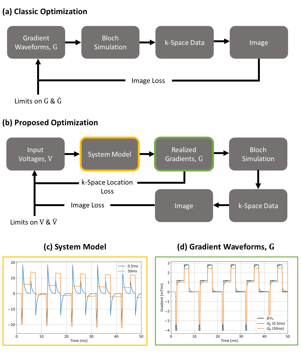
Figure 1: Flowchart of the proposed
pipeline (b) versus a conventional pipeline (a). Eddy current responses
simulated in this work (time constants in legend) are plotted in (c) and
represent the perturbation model used for forward simulation. Corresponding post-perturbation
gradient waveforms ($$$\mathrm{G_0}$$$)
are in (d) and compared to the unperturbed waveform ($$$\beta\mathrm{V_0}$$$).
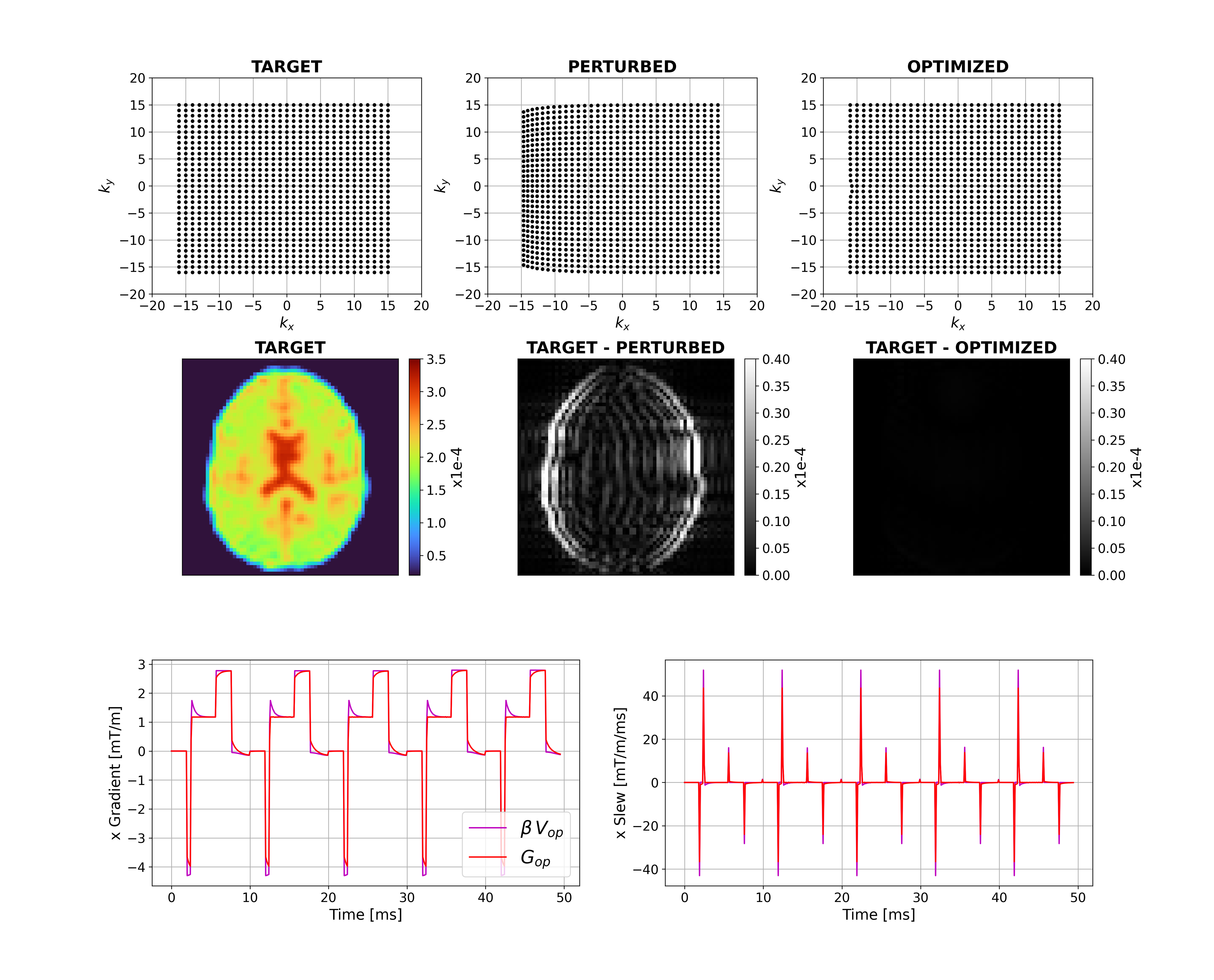
Figure 2: Unconstrained case with a short-term
eddy current. Top row shows k-space trajectories with acquired points
displayed as black dots. The target image is shown on the left-hand side of the
middle row with differences between this and the perturbed and optimized images
alongside. The bottom row shows an example x-gradient and slew rate for the
first 5 TRs. Pre-optimization gradients are in Figure 1 and post-optimization
gradients are shown here (with subscript 'op').
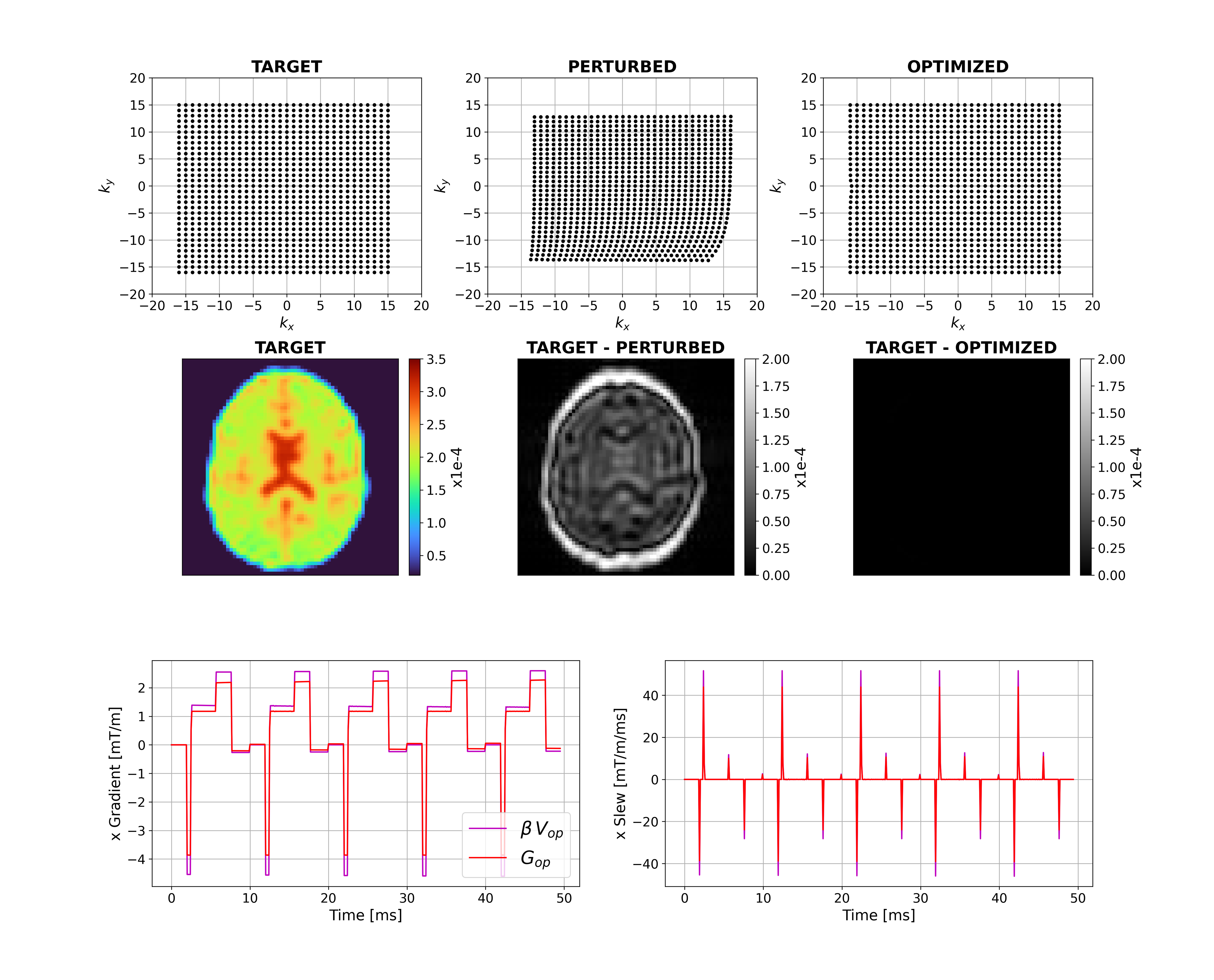
Figure 3: Unconstrained case with a long-term
eddy current. Top row shows k-space trajectories with acquired points
displayed as black dots. The target image is on the left-hand side of the
middle row with differences between this and the perturbed and optimized
images. The bottom row shows example optimal x-gradients and slew rates for the
first 5 TRs.
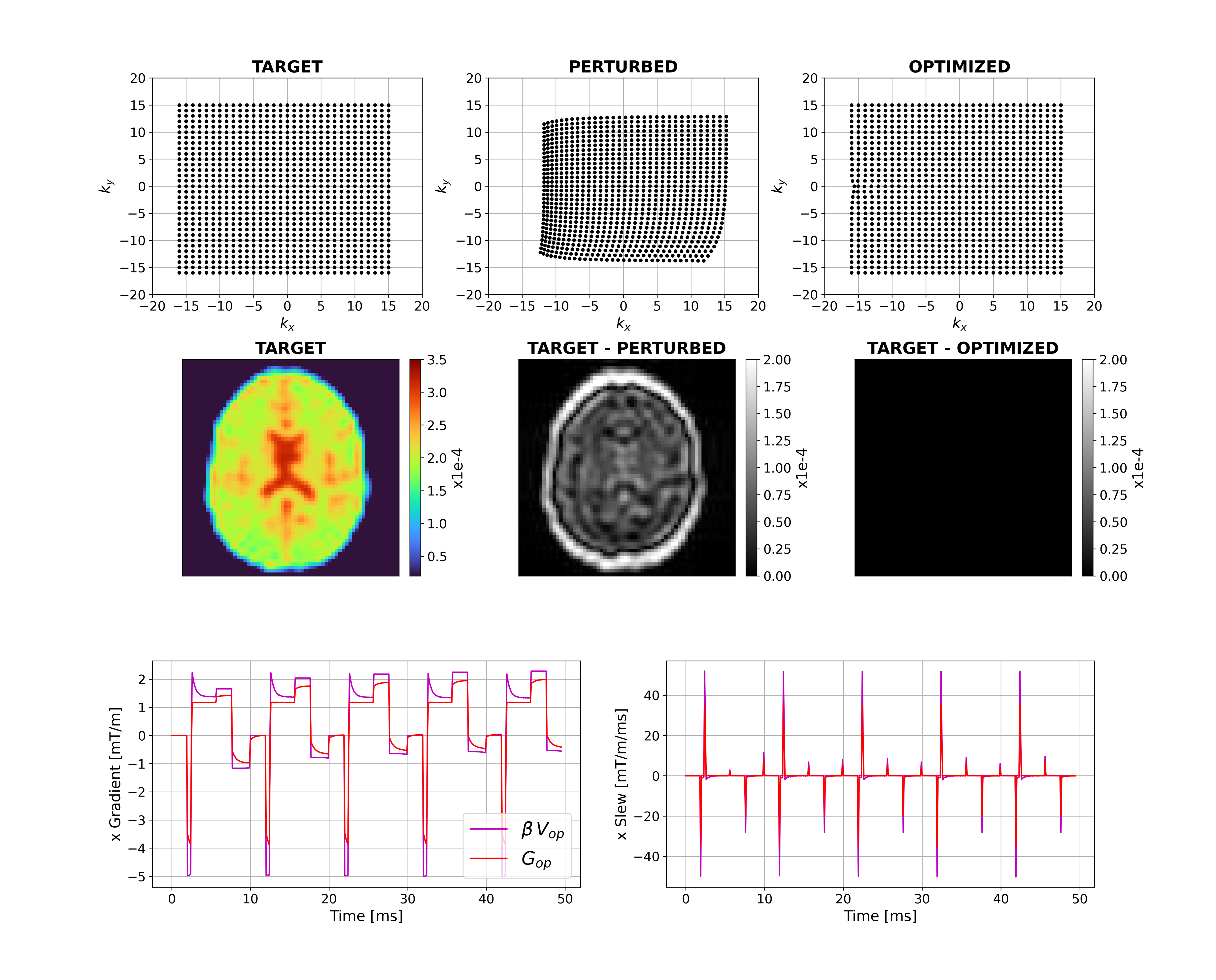
Figure 4: Unconstrained case with short
and long-term eddy currents. Top row shows k-space trajectories with
acquired points displayed as black dots. The target image is on the left-hand
side of the middle row with differences between this and the perturbed and
optimized images. The bottom row shows example optimal x-gradients and slew
rates for the first 5 TRs.
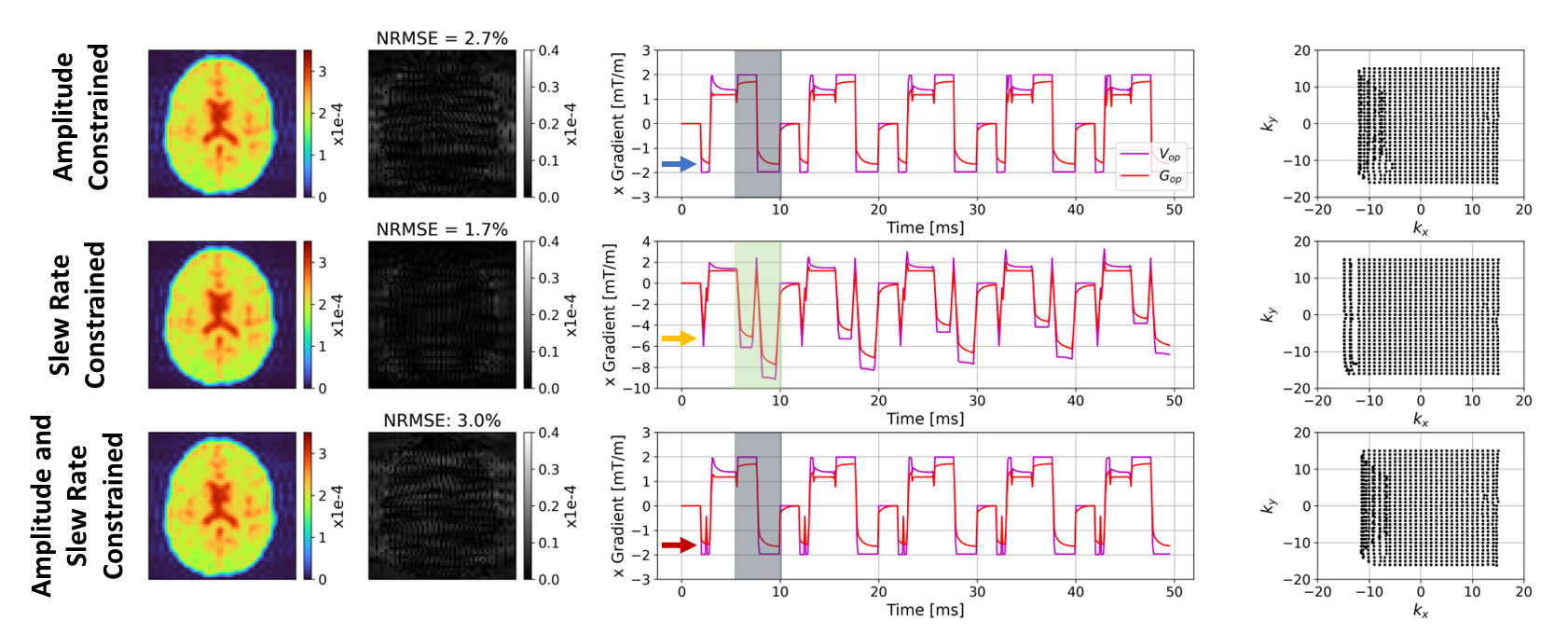
Figure 5: Comparison of results for a bi-exponential
eddy current perturbation with: $$$\beta\mathrm{V_{max}}$$$ = 2mT
(top row), $$$\beta\mathrm{S_{max}}$$$ = 20mT/m/ms (middle row), and $$$\beta\mathrm{V_{max}}$$$ = 2mT and $$$\beta\mathrm{S_{max}}$$$ = 20mT/m/ms (bottom row). $$$\mathrm{I_C}$$$ are on the left, alongside
their differences with respect to $$$\mathrm{I_T}$$$; NRMSEs are
small despite using a set of highly restrictive constraints. Example x-gradients are shown for 5 TRs with respective $$$\mathrm{k_C}$$$ on the right.
DOI: https://doi.org/10.58530/2023/1242