Synopsis

Keywords: Gradients, System Imperfections: Measurement & Correction

Gradient inaccuracies often deteriorate image quality in non-Cartesian MRI, raising a demand for accurate gradient waveform measurements. The recently proposed approach of “variable-prephasing” provides an efficient gradient measurement technique with high SNR. However, the original variable-prephasing sequence neglects lingering field effects from the prephasing gradients, which we show to produce erroneous results if the gradient system exhibits sharp mechanical resonances. We therefore propose “fully compensated variable-prephasing” and demonstrate its ability to remove all field effects not stemming from the test gradient of interest.

Introduction

Non-Cartesian imaging techniques like spiral^1,2 or radial^3–5 often require gradient waveform corrections to obtain good image quality. Recently, a new method for gradient waveform measurements, termed variable-prephasing (VP)⁶, was presented, which efficiently yields gradient progressions with high SNR. We developed an extended method that compensates for concomitant field terms and residual eddy currents from the prephasing gradients and implemented it on a human-sized 7T scanner.

Methods

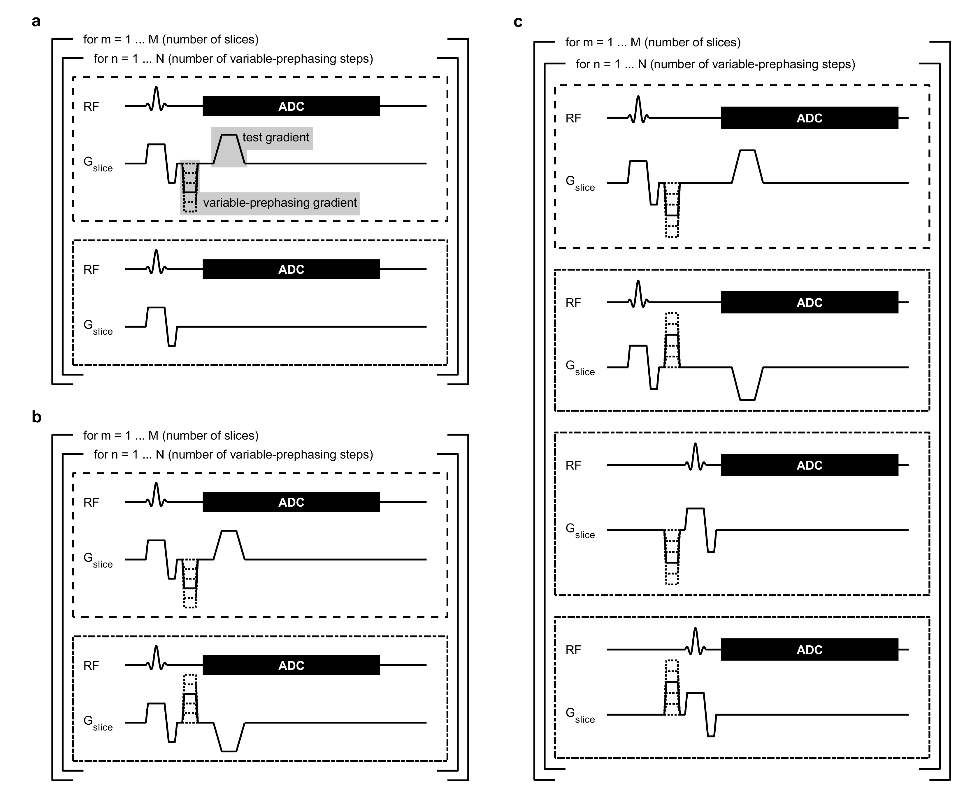
The VP method⁶ constitutes an extension of the thin-slice method⁷ with added prephasing gradients of variable amplitude between the excitation and the test gradient. In the VP method, reference measurements without the prephasing and test gradients are used to compensate for lingering effects of the slice-selection gradient (Figure 1a). Concomitant fields of the test gradient can be compensated for by inverting the signs of the VP and test gradients in the reference measurements, similar to a previously published method⁸ (Figure 1b). In fully compensated variable-prephasing (FCVP), we added two more steps to the sequence, in which the test gradient is off and the slice-selective excitation occurs after the VP gradient, to address lingering gradient distortions caused by the prephasing gradient (Figure 1c).
The field evolution is inferred from the time derivative of the phase of the measured FID signal ($$$f(r,t)$$$). This frequency evolution can be modeled as follows for the four measurements of the n^th VP step in Figure 1c:
$$f_{n,1}(r,t)=\frac{\gamma}{2\pi}\left[\sum_{j=1}^{2}p_j(r)(d_j(t)+d_{j,n}^\text{VP}(t))\right]+c(r,t)+c_n^\text{VP}(r,t)+q^I(r,t)\qquad(1)$$$$\text{with}\quad p_1(r)=1,\quad p_2(r)=r,\quad d_1(t)=\Delta B_0(t),\quad d_2(t)=G(t),\quad d_{1,n}^\text{VP}(t)=\Delta B_{0,n}^\text{VP}(t),\quad d_{2,n}^\text{VP}(t)=G_n^\text{VP}(t)$$
$$f_{n,2}(r,t)=\frac{\gamma}{2\pi}\left[\sum_{j=1}^2p_j(r)(-d_j(t)-d_{j,n}^\text{VP}(t))\right]+c(r,t)+c_n^\text{VP}(r,t)+q^I(r,t)\qquad(2)$$
$$f_{n,3}(r,t)=\frac{\gamma}{2\pi}\left[\sum_{j=1}^2p_j(r)d_{j,n}^\text{VP}(t)\right]+c_n^\text{VP}(r,t)+q^{II}(r,t)\qquad(3)$$
$$f_{n,4}(r,t)=\frac{\gamma}{2\pi}\left[\sum_{j=1}^2p_j(r)(-d_{j,n}^\text{VP}(t))\right]+c_n^\text{VP}(r,t)+q^{II}(r,t)\qquad(4)$$
$$$r$$$ signifies the slice position, $$$p_{\{1,2\}}(r)$$$ represent spatial basis functions⁹ evaluated at position $$$r$$$, $$$d_{\{1,2\}}(t)$$$ and $$$d_{\{1,2\},n}^\text{VP}(t)$$$ are the corresponding field coefficients referring to the test gradient and the n^th VP gradient, respectively. They are explicitly written out in Eq. (1). $$$c(r,t)$$$ and $$$c_n^\text{VP}(r,t)$$$ describe phase contributions due to concomitant fields, while $$$q^I(r,t)$$$ and $$$q^{II}(r,t)$$$ contain background terms originating from the slice selection gradient. Eqs. (1) and (2) are also valid for the sequence depicted in Figure 1b. In the case of Figure 1a, Eq. (2) reduces to $$$f_{n,2}(r,t)=q^I(r,t)$$$.
Stacking the acquisitions from $$$M$$$ different slice positions, we obtain a matrix equation (Eq. (5)) for each time point, which can be solved for $$$d(t)$$$ with the method described by Harkins and Does⁶.
$$\begin{bmatrix}f_{1,1}\\f_{2,1}\\\vdots\\f_{N,1}\\f_{1,2}\\f_{2,2}\\\vdots\\f_{N,2}\\f_{1,3}\\f_{2,3}\\\vdots\\f_{N,3}\\f_{1,4}\\f_{2,4}\\\vdots\\f_{N,4}\end{bmatrix}=\begin{bmatrix}P&P&0&...&0&I_M&0&...&0&0&0&...&0\\P&0&P&...&0&0&I_M&...&0&0&0&...&0\\\vdots&\vdots&\vdots&\ddots&\vdots&\vdots&\vdots&\ddots&\vdots&\vdots&\vdots&\ddots&\vdots\\P&0&0&...&P&0&0&...&I_M&0&0&...&0\\-P&-P&0&...&0&I_M&0&...&0&0&0&...&0\\-P&0&-P&...&0&0&I_M&...&0&0&0&...&0\\\vdots&\vdots&\vdots&\ddots&\vdots&\vdots&\vdots&\ddots&\vdots&\vdots&\vdots&\ddots&\vdots\\-P&0&0&...&-P&0&0&...&I_M&0&0&...&0\\0&P&0&...&0&0&0&...&0&I_M&0&...&0\\0&0&P&...&0&0&0&...&0&0&I_M&...&0\\\vdots&\vdots&\vdots&\ddots&\vdots&\vdots&\vdots&\ddots&\vdots&\vdots&\vdots&\ddots&\vdots\\0&0&0&...&P&0&0&...&0&0&0&...&I_M\\0&-P&0&...&0&0&0&...&0&I_M&0&...&0\\0&0&-P&...&0&0&0&...&0&0&I_M&...&0\\\vdots&\vdots&\vdots&\ddots&\vdots&\vdots&\vdots&\ddots&\vdots&\vdots&\vdots&\ddots&\vdots\\0&0&0&...&-P&0&0&...&0&0&0&...&I_M\end{bmatrix}\,\begin{bmatrix}d\\d_1^\text{VP}\\d_2^\text{VP}\\\vdots\\d_N^\text{VP}\\ c_1^I\\ c_2^I\\\vdots\\c_N^I\\c_1^{II}\\c_2^{II}\\\vdots\\c_N^{II}\end{bmatrix}\qquad(5)$$$$\text{with}\quad f_{n,k}=\begin{bmatrix}f_{n,k}(r_1,t)\\f_{n,k}(r_2,t)\\\vdots\\f_{n,k}(r_m,t)\\\vdots\\f_{n,k}(r_M,t)\end{bmatrix},\quad P=\begin{bmatrix}1&r_1\\1&r_2\\\vdots&\vdots\\1&r_m\\\vdots&\vdots\\1&r_M\end{bmatrix},\quad d=\begin{bmatrix}\Delta B_0(t)\\G(t)\end{bmatrix},\quad d_n^\text{VP}=\begin{bmatrix}\Delta B_{0,n}^\text{VP}(t)\\G_n^\text{VP}(t)\end{bmatrix},$$$$\quad c_n^I=\begin{bmatrix}c(r_1,t)+c_n^\text{VP}(r_1,t)+q^I(r_1,t)\\c(r_2,t)+c_n^\text{VP}(r_2,t)+q^I(r_2,t)\\\vdots\\c(r_m,t)+c_n^\text{VP}(r_m,t)+q^I(r_m,t)\\\vdots\\c(r_M,t)+c_n^\text{VP}(r_M,t)+q^I(r_M,t)\end{bmatrix},\quad c_n^{II}=\begin{bmatrix}c_n^\text{VP}(r_1,t)+q^{II}(r_1,t)\\c_n^\text{VP}(r_2,t)+q^{II}(r_2,t)\\\vdots\\c_n^\text{VP}(r_m,t)+q^{II}(r_m,t)\\\vdots\\c_n^\text{VP}(r_M,t)+q^{II}(r_M,t)\end{bmatrix}$$
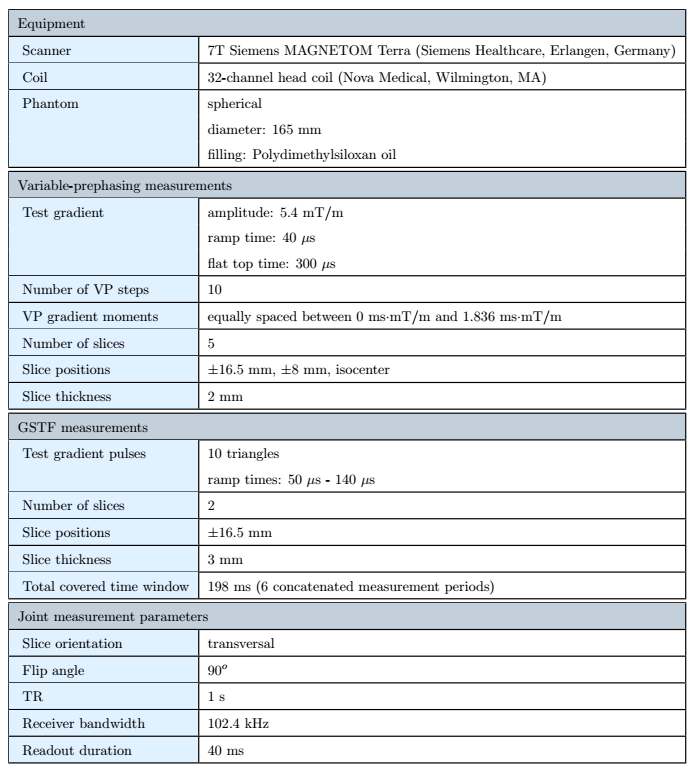
$$$n=1,...,N$$$ is the index of the VP step, $$$m=1,...,M$$$ refers to the slice number, $$$I_M$$$ signifies the identity matrix with $$$M$$$ diagonal elements, and $$$k=1,2,3,4$$$ iterates through the acquisition steps in Figure 1c. We evaluated the obtained gradient progressions by comparing them to calculated ones based on the gradient system transfer function (GSTF)^9–12. Table 1 contains the measurement details.

Results

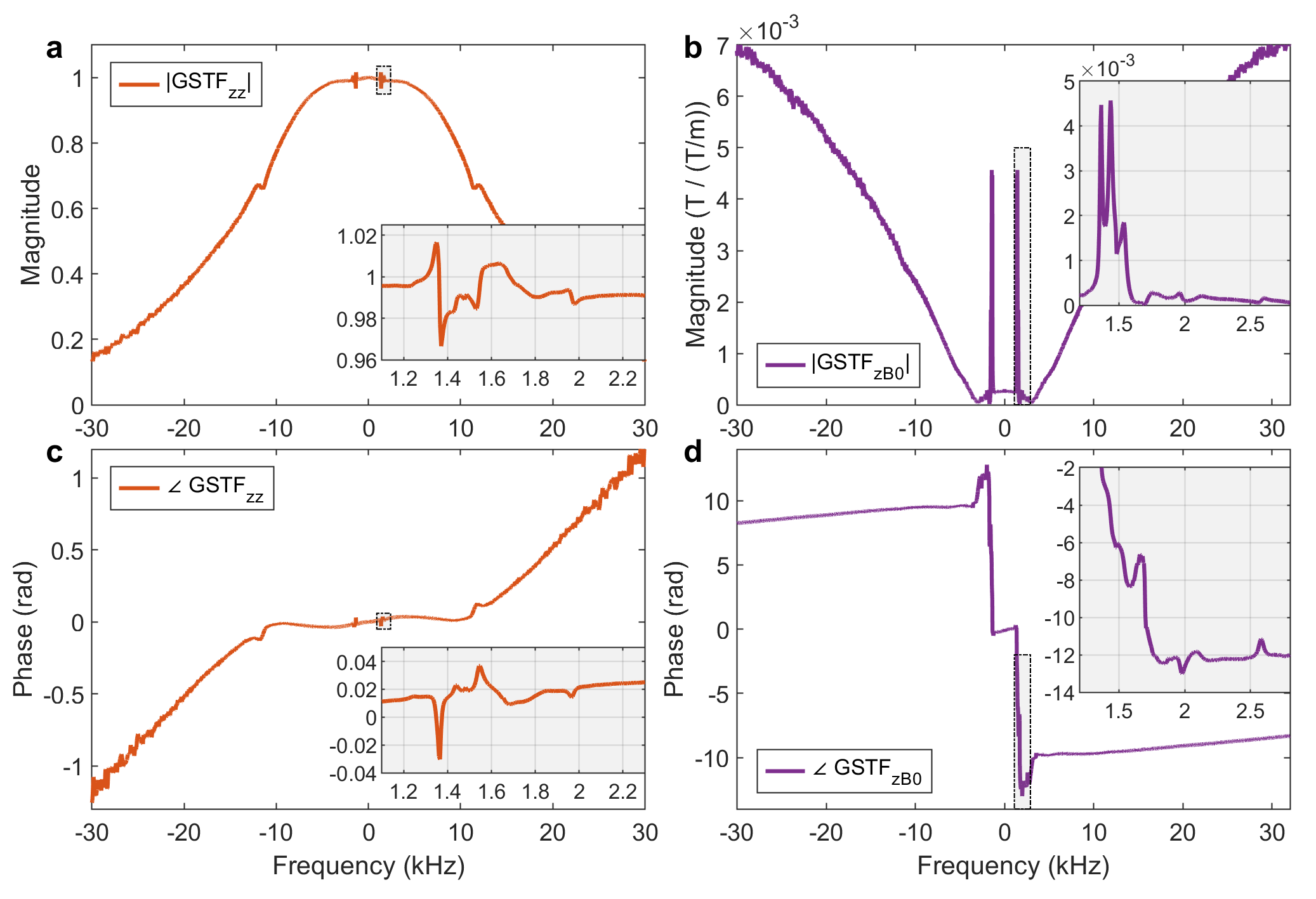
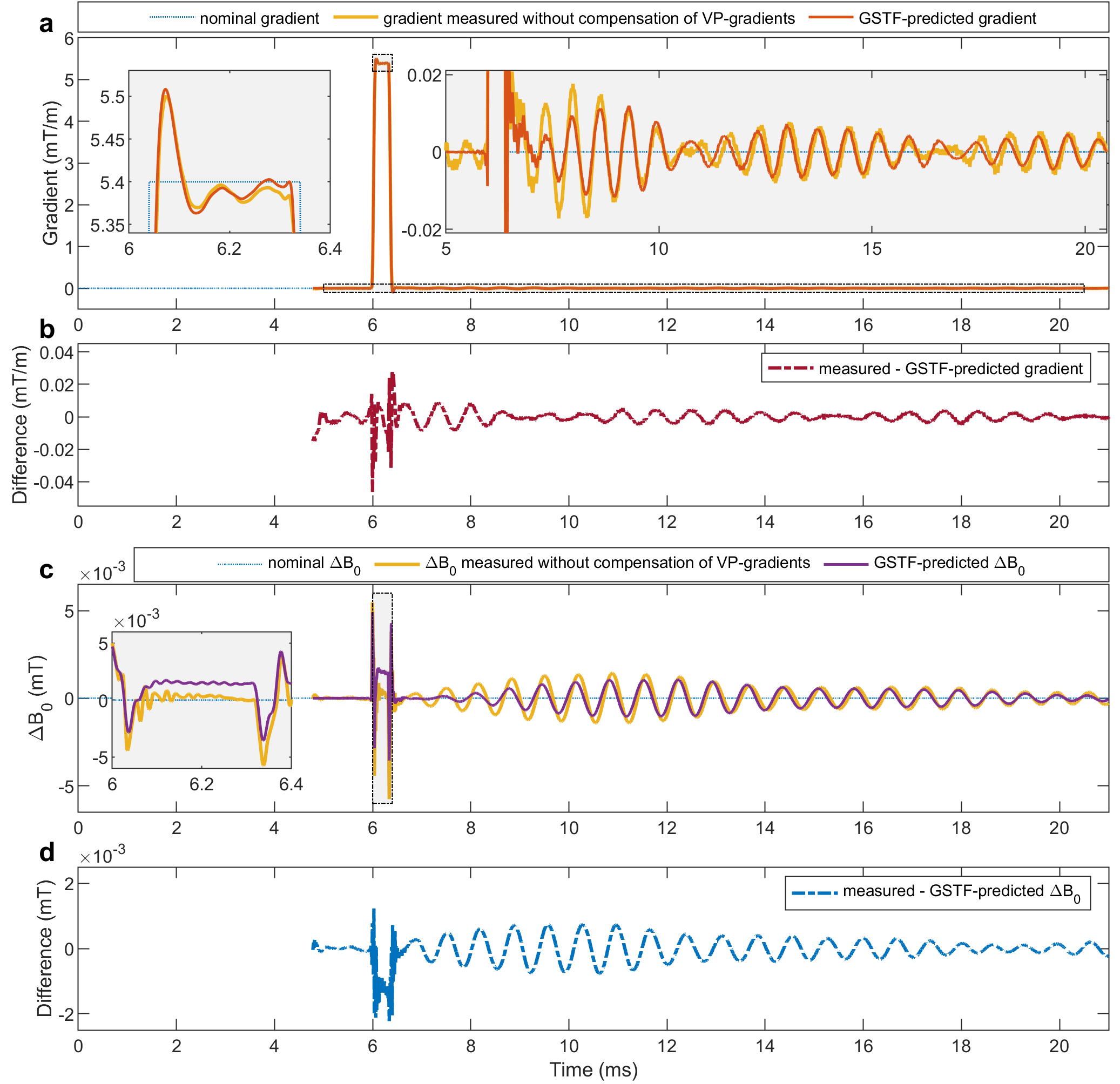
Figure 2 displays the GSTF self-term (a, c) and B₀-cross-term (b, d) of the z-axis of our scanner. The insets feature prominent mechanical resonances.
Figure 3 shows the results of the gradient measurements with the VP sequence compensating for concomitant field effects (cf. Figure 1b). Both the z-gradient (Figure 3a) and the corresponding dynamic B₀-changes (Figure 3c) exhibit considerable lingering field oscillations. Distinct differences between the measured curve and the one predicted by the GSTF are visible. The differences are explicitly plotted in Figure 3b and d, revealing their oscillatory pattern.
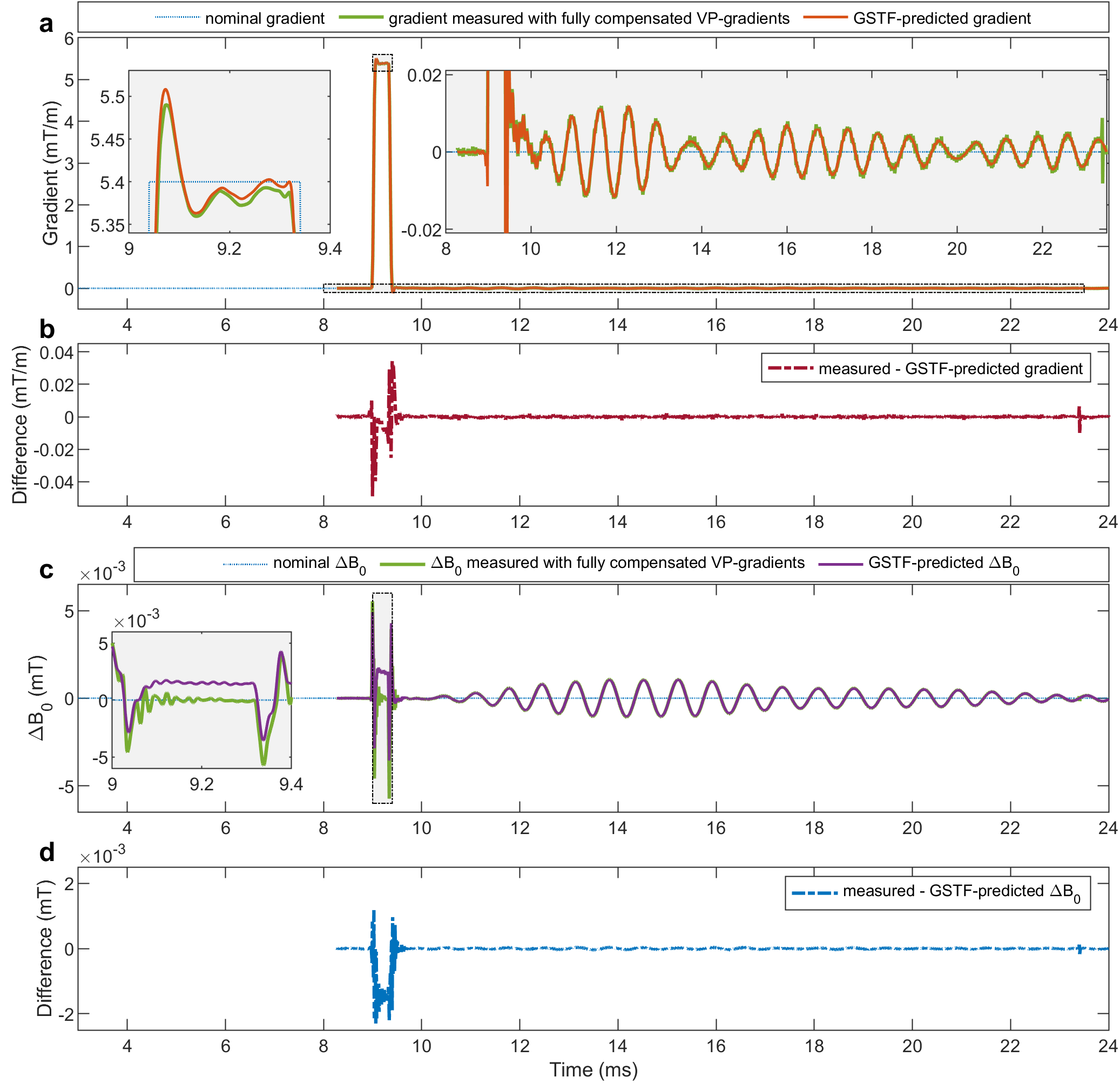
Figure 4 presents the measurement results obtained with the FCVP sequence (cf. Figure 1c). The measured and predicted field evolutions agree much better (Figure 4a, c), which is also reflected in the almost completely flat difference curves (Figure 4b, d). Remaining discrepancies occur at the gradient switching points (Figure 4b, d between 9 ms and 10 ms), and in case of the B₀-changes also during the plateau of the trapezoid (inset in Figure 4c).

Discussion

The oscillations of the gradient and B₀-field after the test gradient reflect the sharp resonance peaks in the GSTF. They arise from mechanical vibrations of the gradient coil. In the right inset in Figure 3a, oscillations of the measured gradient curve before the test gradient can be seen. These oscillations are the repercussions of the VP gradient, averaged over the different VP steps. The difference plots in Figure 3b and d reveal how they are superimposed on the field distortions caused by the test gradient alone. Since the GSTF-based calculation is ignorant of the VP gradients, it does not replicate their lingering effects. With our proposed fully compensated measurement scheme (Figure 1c), the effects from the VP gradients are successfully removed from the measured field evolution (Figure 4). Since the GSTF relies on the assumption that the gradient system is linear and time-invariant, non-linear characteristics of the gradient amplifiers cause the measured curves to differ from the ones predicted by the GSTF-model¹³. This is supposedly the reason for the remaining discrepancies observed in Figure 4.

Conclusion

Variable-prephasing is a potent method for accurate measurements of gradient field progressions without being limited by the signal dephasing induced by the test gradient. However, on scanners whose gradient coils exhibit strong mechanical resonances causing long-living lingering field distortions, it is important to compensate the effects of the prephasing gradients. The FCVP sequence we present here thus offers a simple, effective measurement technique applicable on a wide range of hardware setups.

Acknowledgements

No acknowledgement found.

References

1. Tan H, Meyer CH. Estimation of k -space trajectories in spiral MRI. Magn Reson Med. 2009;61(6):1396-1404. doi:10.1002/mrm.21813

2. Robison RK, Devaraj A, Pipe JG. Fast, simple gradient delay estimation for spiral MRI. Magn Reson Med. 2010;63(6):1683-1690. doi:10.1002/mrm.22327

3. Deshmane A, Blaimer M, Breuer F, et al. Self‐calibrated trajectory estimation and signal correction method for robust radial imaging using GRAPPA operator gridding. Magn Reson Med. 2016;75(2):883-896. doi:10.1002/mrm.25648

4. Krämer M, Biermann J, Reichenbach JR. Intrinsic correction of system delays for radial magnetic resonance imaging. Magn Reson Imaging. 2015;33(4):491-496. doi:10.1016/j.mri.2015.01.005

5. Moussavi A, Untenberger M, Uecker M, Frahm J. Correction of gradient-induced phase errors in radial MRI. Magn Reson Med. 2014;71(1):308-312. doi:10.1002/mrm.24643

6. Harkins KD, Does MD. Efficient gradient waveform measurements with variable-prephasing. Journal of Magnetic Resonance. 2021;327:106945. doi:10.1016/j.jmr.2021.106945

7. Duyn JH, Yang Y, Frank JA, van der Veen JW. Simple Correction Method fork-Space Trajectory Deviations in MRI. Journal of Magnetic Resonance. 1998;132(1):150-153. doi:10.1006/jmre.1998.1396

8. Brodsky EK, Klaers JL, Samsonov AA, Kijowski R, Block WF. Rapid measurement and correction of phase errors from B0 eddy currents: Impact on image quality for non-cartesian imaging. Magn Reson Med. 2013;69(2):509-515. doi:10.1002/mrm.24264

9. Vannesjo SJ, Haeberlin M, Kasper L, et al. Gradient system characterization by impulse response measurements with a dynamic field camera. Magn Reson Med. 2013;69(2):583-593. doi:10.1002/mrm.24263

10. Addy NO, Wu HH, Nishimura DG. Simple method for MR gradient system characterization and k-space trajectory estimation. Magn Reson Med. 2012;68(1):120-129. doi:10.1002/mrm.23217

11. Scholten H, Stich M, Köstler H. Phantom-based high-resolution measurement of the gradient system transfer function. In: Proceedings of the 2021 ISMRM Annual Meeting. Abstract number 3087; 2021.

12. Wilm BJ, Dietrich BE, Reber J, Johanna Vannesjo S, Pruessmann KP. Gradient Response Harvesting for Continuous System Characterization during MR Sequences. IEEE Trans Med Imaging. 2020;39(3):806-815. doi:10.1109/TMI.2019.2936107

13. Rahmer J, Schmale I, Mazurkewitz P, Lips O, Börnert P. Non‐Cartesian k‐space trajectory calculation based on concurrent reading of the gradient amplifiers’ output currents. Magn Reson Med. 2021;85(6):3060-3070. doi:10.1002/mrm.28725