1228
Accelerating beyond the sound limit: Ultrasonic Wave-CAIPI using a dual-axis head gradient insert1Department of High Field MR Research, University Medical Center Utrecht, Utrecht, Netherlands, 2Spinoza centre for Neuroimaging, Amsterdam, Netherlands
Synopsis
Keywords: Gradients, New Trajectories & Spatial Encoding Methods, Ultrasonic
In this work, we present peripheral nerve stimulation and imaging results for a dual-axis head gradient that operates at ultrasonic frequencies. PNS measurements on 4 volunteers did not yield any noticeable stimulation. Imaging was performed using an ultrasonic Wave-CAIPI MP-RAGE, which featured ~20-fold acceleration and fully-sampled K-space coverage. We show the first images with this approach and a g-factor close to unity.Introduction
Acceleration techniques like Wave-CAIPI use rapidly oscillating gradients during the readout to enable high acceleration factors, with minimal g-factor penalty on SNR1. The reduced g-factors are a result of the additional spatial encoding provided by the oscillating gradients. Previously, we demonstrated decreased g-factors of Wave-CAIPI when using high-amplitude waves on a single-axis gradient insert2. However, these gradient waves generate significant additional acoustic noise, which increases linearly with amplitude, to the extent that it limited the in-vivo attainable amplitude.Acoustic noise can be lowered by reducing the slew rates of gradients3, but that results in longer scan times. Alternatively, switching the gradients faster, above 20 kHz, produces ultrasonic inaudible noise4,5. We previously demonstrated this concept using a gradient insert with a single-axis, that limited scan directions and maximum acceleration.
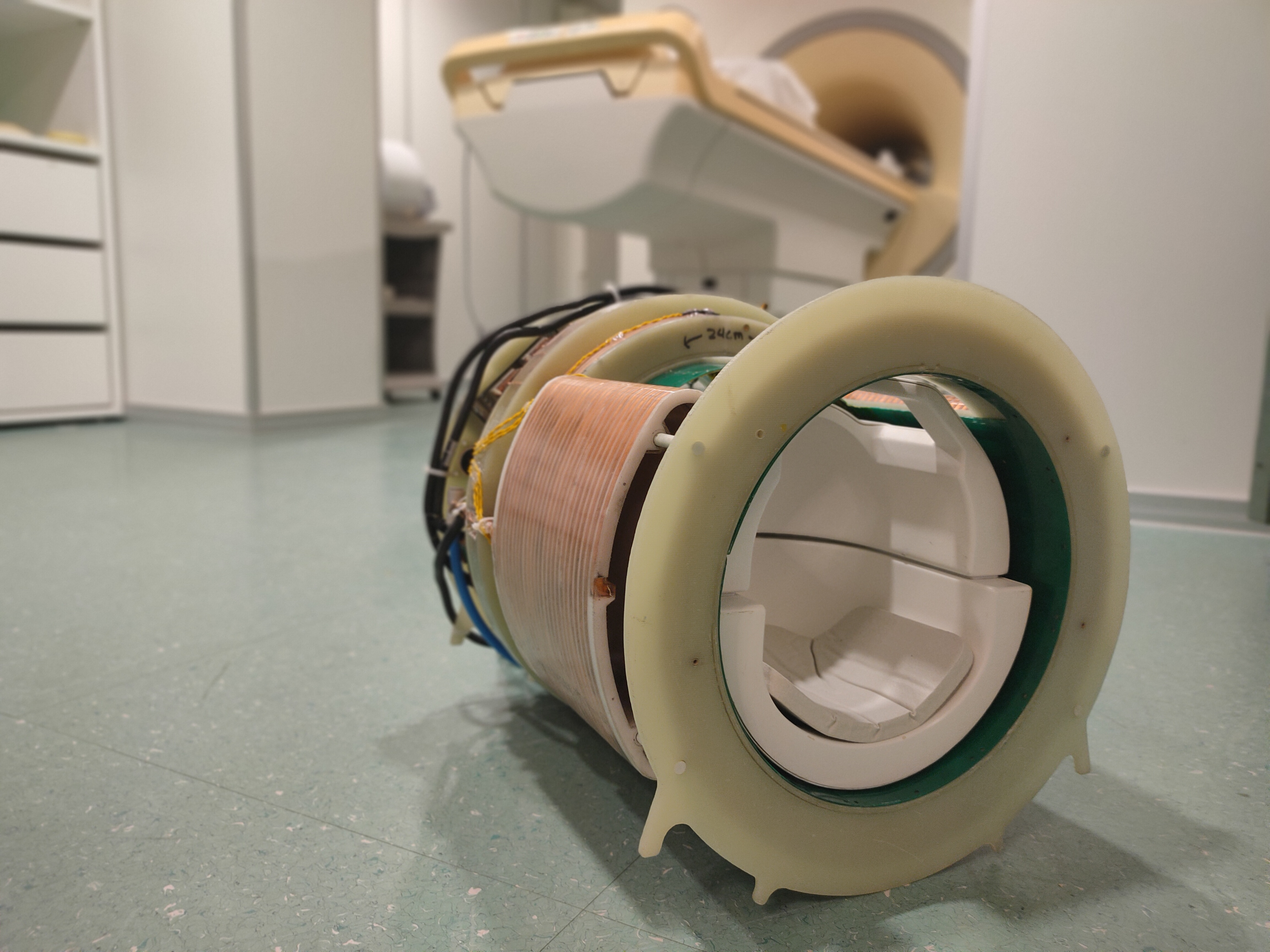
This work demonstrates the acoustic noise and peripheral nerve stimulation (PNS) characteristics of a novel ultrasonic dual-axis gradient insert, as depicted in figure 1. We show the first in-vivo images and quiet acceleration potential of ultrasonic Wave-CAIPI using this insert gradient.
Methods
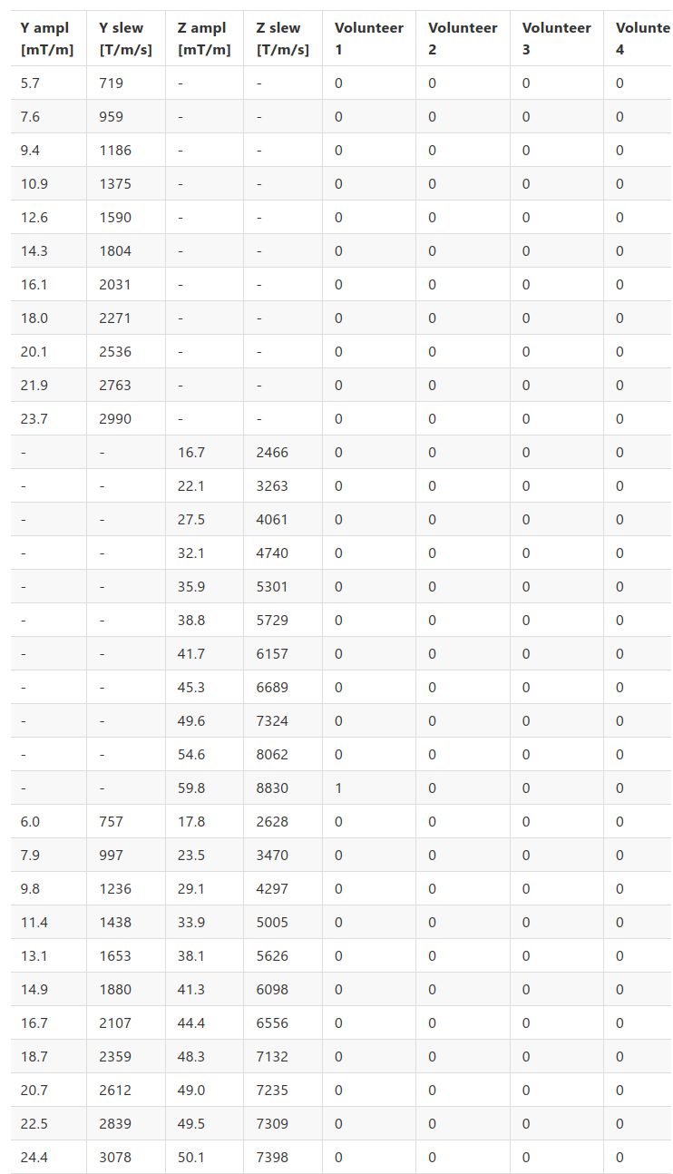
The head gradient features Z- & Y-coils, and matching capacitor banks for resonance at 23.5 and 20.8 kHz, respectively. A modified gradient amplifier (Prodrive) drives the gradients through an open Faraday cage. The gradient is fitted with an ultra-thin 8-channel transmit dipole array7 and 32-channel receive array (Nova Medical). The gradient was placed in a 7T MR-scanner (Philips) for all experiments.The PNS characteristics of the coils were investigated on four healthy subjects (3 male, aged 22-51). Three sets of incrementally increasing amplitudes were studied, one of each coil individually and one combined. Four pulse-trains of 50ms were played out at each gradient amplitude, which the subjects scored for PNS sensations on a scale from 1 (very slight) to 5 (painfull). Sound was measured using a calibrated condenser microphone (Behringer) placed in the gradient insert. Exponential filtering and A-weighting was applied to compute sound levels.
A quiet (76dB) MP-RAGE sequence, with reduced slew-rate and amplitude, was used to investigate the acceleration potential6. It features a whole-brain FOV of 304x192x256mm at 1mm3 resolution, with TR/TE/α/BW = 18ms / 8.88ms / 13° / 155 Hz/px. Acceleration factors of 2.9 (Y-direction) and 6.6 (Z-direction) reduce the scan duration to 53 seconds. The scan is acquired with CAIPI and Wave-CAIPI at amplitudes of 24 mT/m (Y) and 50 mT/m (Z).
Reconstruction is performed by a NUFFT-based pipeline using MATLAB, MRecon (GyroTools) and BART8. The trajectory is computed by merging the GIRF-corrected9 waveforms of the whole-body gradients and the oscillating gradients captured by a PSF scan1. Sensitivity maps are calculated using ESPIRiT10 on a low-resolution reference acquisition. 12 iterations of CG-SENSE11 with L1-regularisation produce the final reconstruction.
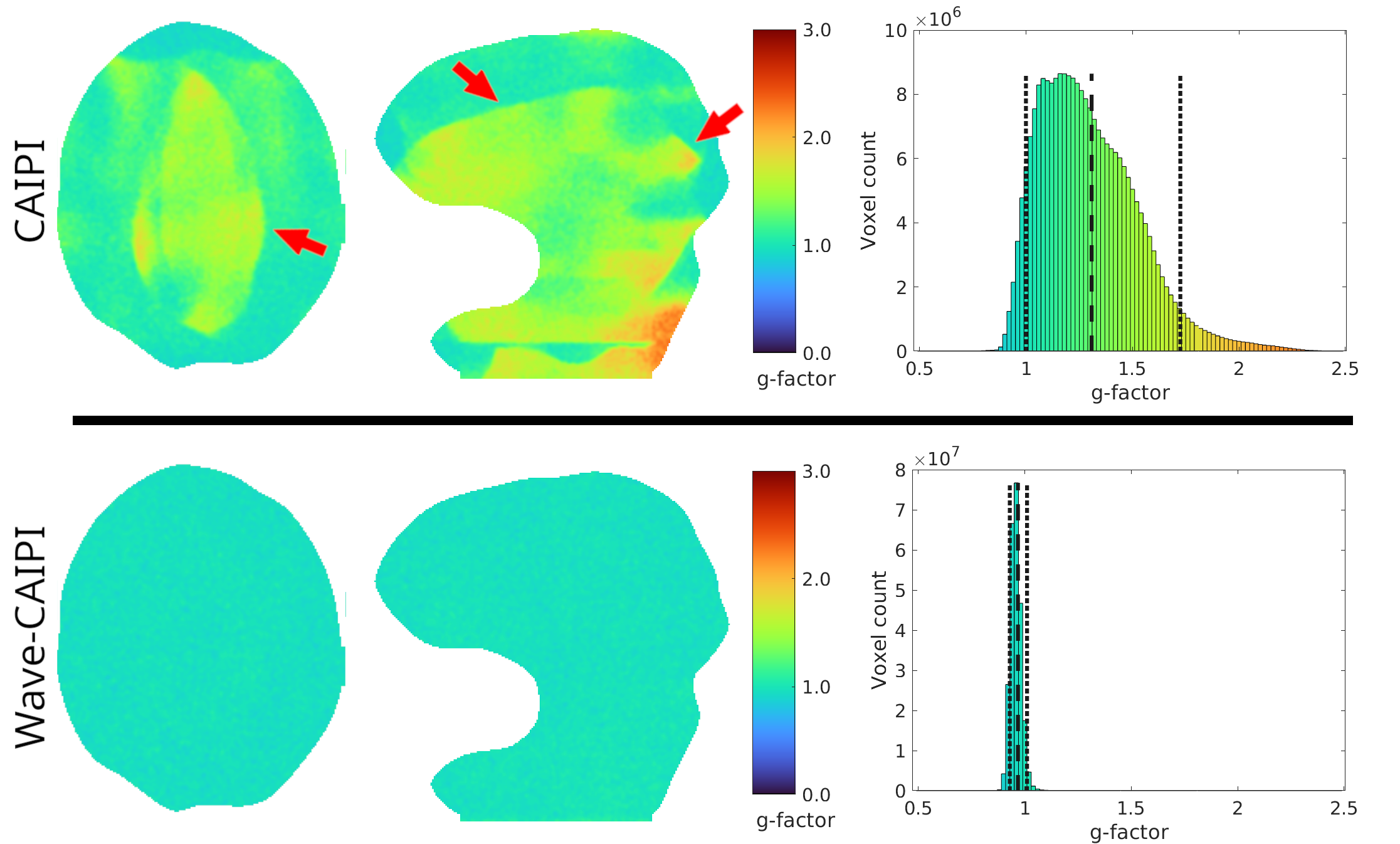
Finally, g-factor maps were computed for both acquisitions using the pseudo multiple replica method12 that performed the entire reconstruction 50 times with additional simulated noise.
Results
The PNS experiences over the three amplitude sweeps are shown in the table of figure 2. A single weak PNS experience was reported by one of the volunteers at 60 mT/m, 10 mT/m above that utilized in the Wave-CAIPI encoding.When both coils produce their ultrasonic frequencies, an audible beat tone is produced. The sound level of this tone was measured at 93dB.
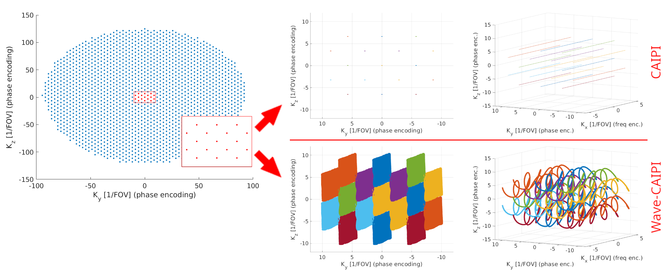
The trajectories through K-space, and specially the impact of the addition of waves, are depicted in figure 3. The Wave-CAIPI readouts contain a cuboid-like area that leaves little unsampled voids, contrary to the straight lines of CAIPI.
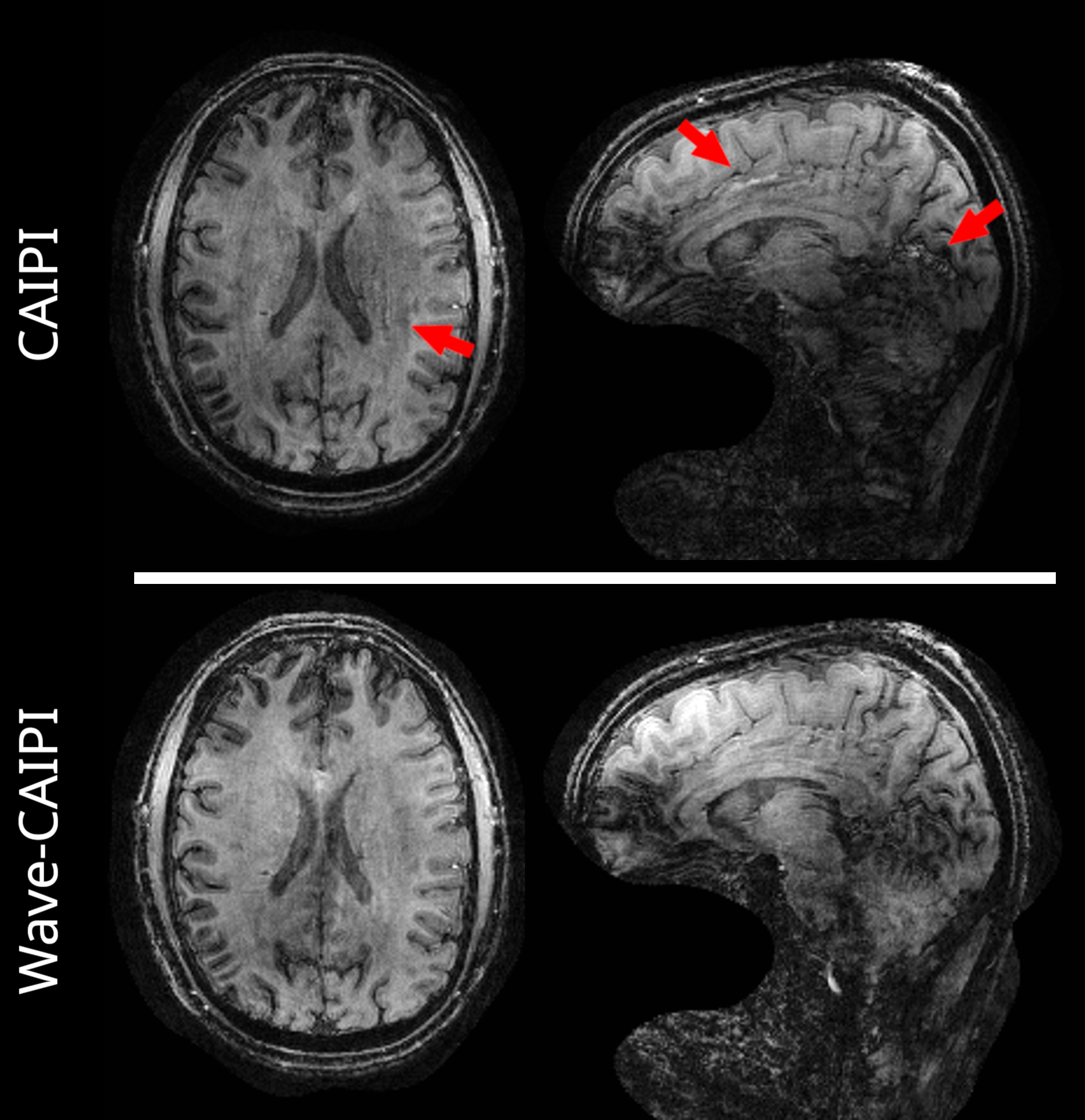
Figure 4 shows the reconstructed MP-RAGE for both acquisition types. While both scans show B1+ imhomogeneities with a spatially varying intensity and contrast, the Wave-CAIPI acquisition shows reduced artifacts due to acceleration.
The g-factors over the previously depicted slices are shown in figure 5, next to histograms computed over the entire brain. While the CAIPI acquisition shows a pattern of elevated g-factors with a mean of 1.3, this factor is very close to 1.0 when using Wave-CAIPI.
Discussion
The presented ultrasonic in-vivo scans are, despite the almost 20-fold acceleration, fully-sampled by the additional encoding provided by the dual-axis insert gradient. Similar to regular fully-sampled scans, there is no g-factor penalty.Since a clear PNS limit is not reached yet, amplitudes could be increased further, to render acceleration factors beyond 20x similarly fully-sampled.
Further improvements in image quality are possible by mitigating the B1-imhomogeneity with improved RF-pulses, such as Kt-points7.
The beat tone renders the ultrasonic encoding not fully inaudible, but the measured sound level at 93dB is significantly lower than the measured sound level for conventional encoding.
Although we used a quiet scan, the technique can also be used with traditional (loud) accelerated scans, such as EPI. While obtaining sufficient wave-induced spreading for a optimal g-factor reduction in scans with high pixel bandwiths may not be possible with conventional gradient-systems, they likely are with the presented ultrasonic insert gradient.
Conclusion
The demonstrated usage of an insert gradient transforms K-space lines into K-space cuboids, making highly accelerated (~20x) scans fully sampled, resulting in PNS-free and quiet acceleration without g-factor penalty and thus optimal SNR.Acknowledgements
We gratefully acknowledge funding of the Dutch Research Counsil; NWO-VIDI 18361-WijnenReferences
1. Bilgic B, Gagoski BA, Cauley SF, et al. Wave-CAIPI for highly accelerated 3D imaging. Magn. Reson. Med. 2015;73:2152–2162 doi: 10.1002/mrm.25347.
2. Roos THM, Versteeg E, Siero JC. Ultra-high field done ultra-fast: Enhancing Wave-CAIPI using an single-axis insert head gradient. In: Proceedings of the 30th Annual Meeting of ISMRM. ; 2022. p. #0505.
3. Hennel F, Girard F, Loenneker T. “Silent” MRI with soft gradient pulses. Magn. Reson. Med. 1999;42:6–10 doi: 10.1002/(SICI)1522-2594(199907)42:1<6::AID-MRM2>3.0.CO;2-D.
4. Versteeg E, Klomp DWJ, Siero JCW. A silent gradient axis for soundless spatial encoding to enable fast and quiet brain imaging. Magn. Reson. Med. 2022;87:1062–1073 doi: 10.1002/mrm.29010.
5. Versteeg E, Klomp DWJ, Siero JCW. Accelerating Brain Imaging Using a Silent Spatial Encoding Axis. Magn. Reson. Med. 2022:1–9 doi: 10.1002/mrm.29350.
6. Jacobs SM, Versteeg E, van der Kolk AG, et al. Image quality and subject experience of quiet T1-weighted 7-T brain imaging using a silent gradient coil. Eur. Radiol. Exp. 2022 61 2022;6:1–9 doi: 10.1186/S41747-022-00293-X.
7. Roos THM, Gosselink WJM, Bensink M, et al. Ultra-thin dipole array for uniform B1+in silent dual-axis insert head gradient. ISMRM Workshop on Ultra-High Field MR; 2022
8. Uecker M, Ong F, Tamir JI, et al. Berkeley Advanced Reconstruction Toolbox. Annual Meeting ISMRM, Toronto 2015, In: Proc. Intl. Soc. Mag.Reson. Med 2015;23:2486.
9. Vannesjo, Signe J., et al. "Gradient system characterization by impulse response measurements with a dynamic field camera." Magneticresonance in medicine 69.2 (2013): 583-593.
10. Uecker, Martin, et al. "ESPIRiT—an eigenvalue approach to autocalibrating parallel MRI: where SENSE meets GRAPPA." Magnetic resonancein medicine 71.3 (2014): 990-1001.
11. Pruessmann, Klaas P., et al. "Advances in sensitivity encoding with arbitrary k‐space trajectories." Magnetic Resonance in Medicine: An Official Journal of the International Society for Magnetic Resonance in Medicine 46.4 (2001): 638-651.
12. Robson, Philip M., et al. "Comprehensive quantification of signal‐to‐noise ratio and g‐factor for image‐based and k‐space‐based parallel imaging reconstructions." Magnetic Resonance in Medicine: An Official Journal of the International Society for Magnetic Resonance inMedicine 60.4 (2008): 895-907.
Figures