1190
In vivo multimodal MRI of the healthy optic nerves
Antonio Ricciardi1, Marios C. Yiannakas1, Ratthaporn Boonsuth1, Rodas Ghilom Bogatsion1, Claudia A. M. Gandini Wheeler-Kingshott1,2,3, and Rebecca S. Samson1
1NMR Research Unit, Queen Square Multiple Sclerosis Centre, UCL Queen Square Institute of Neurology, Faculty of Brain Sciences, University College London, London, United Kingdom, 2Department of Brain and Behavioural Sciences, University of Pavia, Pavia, Italy, 3Brain Connectivity Research Center, IRCCS Mondino Foundation, Pavia, Italy
1NMR Research Unit, Queen Square Multiple Sclerosis Centre, UCL Queen Square Institute of Neurology, Faculty of Brain Sciences, University College London, London, United Kingdom, 2Department of Brain and Behavioural Sciences, University of Pavia, Pavia, Italy, 3Brain Connectivity Research Center, IRCCS Mondino Foundation, Pavia, Italy
Synopsis
Keywords: Nerves, Quantitative Imaging
The optic nerve (ON) is implicated in a variety of neurological disorders but is challenging to study through magnetic resonance imaging due to its small size and jittering. In this study, we developed an acquisition protocol and analysis pipeline that enables to produce quantitative proton density (PD), macromolecular tissue volume (MTV), T2* and T1 maps of the ON from a 20-minute scan. Results show good scan-rescan reproducibility of ON values, and agreement with regional brain values. Significant differences in PD, MTV and T1 were observed between left-right ON measures, and left-right fronto-temporal white matter, which warrant further investigation.Introduction
The optic nerve (ON) may be affected by a variety of neurological disorders1, with magnetic resonance imaging (MRI) having played a key role in their clinical assessment, e.g. optic neuritis, often associated with multiple sclerosis2, and glaucoma3. Quantitative MRI techniques can be employed to estimate biophysical parameters such as relaxometry and myelin concentration, hence detecting subtle alterations otherwise invisible to conventional acquisitions. Despite its potential, the use of MRI to study the ON pathophysiology is still largely unexplored. The small ON calibre requires high cross-sectional resolution to minimise partial volume effects with the surrounding fluid and orbital fat. Furthermore, MRI of the ON is affected by susceptibility induced artifacts due to the adjacent sinuses’ air cavities, and blurring caused by involuntary eye jittering4.In this pilot study, a 20-minute multimodal MRI protocol was developed to optimise the quantitative mapping of: i) proton density (PD), ii) macromolecular tissue volume (MTV), iii) T2*, and iv) T1 relaxation times in the ON. PD and MTV ($$$\text{MTV}=1-\text{PD}$$$), in particular, have been shown to provide consistent proxy estimates of axonal myelination in the brain5.
Methods
Cohort and MRI acquisition. The cohort consisted of 10 healthy volunteers (5 males, aged 20-60 years), scanned on a 3T Philips Ingenia CX MR system, 6 of whom were rescanned to assess repeatability . All acquisitions were performed over a 180x66x180mm3 field of view (FOV) prescribed in the coronal plane, orthogonal to the ON longitudinal axis, covering the entire length of the ON, chiasm, and frontal brain. The MRI protocol included: 1) 2D fat-suppressed T1-weighted inversion recovery (IR) turbo spin-echo (TSE) (flip angle: 90°; echo-time (TE): 10ms, repetition time (TR): 2350ms, inversion delay time: 1000ms, TSE-factor: 11; resolution: 0.5x0.5x2mm3) for both brain and ON segmentation; 2) multi-echo 3D spoiled gradient-echo (SPGR) (flip angle: 24°; 6 echoes, TE1 /ΔTE: 2.5/4.2ms, TR: 35ms; resolution: 0.5x0.5x3mm3); 3) 3D SPGR (flip angle: 4°; TE: 2.6ms, TR: 2.5ms; resolution: 0.5x0.5x3mm3); 4) dual-TR 3D gradient-echo (flip angle: 60°; TE: 2.6ms, TR: 30/180ms; resolution: 2x2x6mm3) for B1 mapping.Preprocessing. Segmentation of white matter (WM), cortical grey matter (cGM) and deep grey matter (dGM) was performed on the IR-TSE images using Geodesic Information Flows (GIF)6. GIF failed on 2 scans and 1 rescan; for these cases, segmentation was performed using FSL7 with manual adjustments. ON left and right masks were delineated manually over the IR-TSE images for all scans, and rigidly registered onto the rescan to test repeatability. Left and right fronto-temporal WM masks - same coronal slices as the ON - were also produced. Segmented data and ON masks were then rigidly registered to the SPGR space using NiftyReg8. Images in SPGR space were cropped to remove the two most anterior and posterior coronal slices due to signal inhomogeneities at the FOV boundary.
Image analysis. Image processing was performed using the MyRelax toolbox9. A B1 map was calculated from the dual-TR gradient-echo images in native space via actual flip angle imaging10, registered to SPGR space and cropped. Quantitative PD, MTV, T2*, and T1 maps were then extracted.
Statistical analysis. Mean values of all quantitative metrics were calculated in WM, left and right fronto-temporal WM, cGM, dGM, and left, right and total ON, after excluding outlier voxels, using MATLAB-202011. Paired t-tests were performed across left and right ON and fronto-temporal WM values to assess laterality. To evaluate repeatability, coefficients of variation (CV) for all metrics in mean, left, right ON, WM, cGM and dGM were calculated as the root mean square across the $$$n=6$$$ subjects CV’s12:
$$\text{CV} = \sqrt{\frac{1}{n}\sum_{i=1}^n \text{CV}_i^2} = \sqrt{\frac{1}{n}\sum_{i=1}^n\frac{\sigma_i^2}{\mu_i^2}}$$
where $$$\text{CV}_i$$$, $$$\sigma_i^2=\frac{(x_i^\text{scan}-x_i^\text{rescan})^2}{2}$$$ and $$$\mu_i=\frac{x_i^\text{scan}-x_i^\text{rescan}}{2}$$$ are the $$$i$$$-th subject's CV, variance and mean between scan-rescan regional values $$$x_i$$$, respectively. Statistical analyses were performed using Scipy13 in Python 3.9.1314.
Results
An overview of PD, MTV, T2* and T1 quantitative maps, together with ON, WM, cGM and dGM masks, is displayed in Figure 1. Distributions of regional values are shown in Figure 2. Laterality tests are reported in Figure 3, with significant differences observed in PD ($$$p=0.003$$$), MTV ($$$p=0.003$$$) and T1 ($$$p=0.031$$$) between left and right ON; the same significant trends were observed between left-right fronto-temporal WM ($$$p=0.026$$$, $$$p=0.026$$$, $$$p=0.025$$$, respectively). CV scores are reported in Table 1, with CVs below 10% observed for all metrics and all tissues except for MTV, where CV of up to 28% was calculated.Discussion
Significant laterality in PD, MTV and T1 values in the ON can be related to an overall skewed distribution, as the same behaviour was also observed in the fronto-temporal WM. Further studies - both in vivo and in phantoms - are required to assess whether this result is physiologically grounded, spurious, or method-related (e.g. due to bias-field). CV results showed an acceptable degree of test-retest reproducibility. Since $$$\text{MTV}=1-\text{PD}$$$ is directly derived from PD, it inherits its variance whilst having lower mean values. This explains the higher CV scores, and suggests MTV reproducibility should be interpreted through PD. Overall, we presented a multimodal MRI acquisition and processing pipeline for the extraction of quantitative PD, MTV, T2* and T1 maps in the ON, which is consistent with the behaviour of the same metrics in other brain tissues in terms of average values and repeatability.Acknowledgements
This project has received funding under the European Union’s Horizon2020 (Human Brain Project SGA3, Specific Grant Agreement No. 945539), BRC (#BRC704/CAP/CGW), MRC (#MR/S026088/1), Ataxia UK, MS Society (#77), Wings for Life (#169111), CureDRPLA, and we thank the UCL-UCLH Biomedical Research Centre for ongoing support. CGWK is a shareholder in Queen Square Analytics Ltd.References
- Selhorst, J.B. and Chen, Y., 2009, February. The optic nerve. In Seminars in neurology (Vol. 29, No. 01, pp. 029-035). Thieme Medical Publishers.
- Toosy, A.T., Mason, D.F. and Miller, D.H., 2014. Optic neuritis. The Lancet Neurology, 13(1), pp.83-99.
- Wang, J., Li, T., Sabel, B.A., Chen, Z., Wen, H., Li, J., Xie, X., Yang, D., Chen, W., Wang, N. and Xian, J., 2016. Structural brain alterations in primary open angle glaucoma: a 3T MRI study. Scientific reports, 6(1), pp.1-9.
- Hoch, M.J., Bruno, M.T. and Shepherd, T.M., 2017. Advanced MRI of the optic nerve. Journal of Neuro-Ophthalmology, 37(2), pp.187-196.
- Mezer, A., Yeatman, J.D., Stikov, N., Kay, K.N., Cho, N.J., Dougherty, R.F., Perry, M.L., Parvizi, J., Hua, L.H., Butts-Pauly, K. and Wandell, B.A., 2013. Quantifying the local tissue volume and composition in individual brains with magnetic resonance imaging. Nature medicine, 19(12), pp.1667-1672.
- Cardoso, M.J., Modat, M., Wolz, R., Melbourne, A., Cash, D., Rueckert, D. and Ourselin, S., 2015. Geodesic information flows: spatially-variant graphs and their application to segmentation and fusion. IEEE transactions on medical imaging, 34(9), pp.1976-1988.
- Andersson, J.L. and Sotiropoulos, S.N., 2016. An integrated approach to correction for off-resonance effects and subject movement in diffusion MR imaging. Neuroimage, 125, pp.1063-1078.
- Modat, M., Ridgway, G.R., Taylor, Z.A., Lehmann, M., Barnes, J., Hawkes, D.J., Fox, N.C. and Ourselin, S., 2010. Fast free-form deformation using graphics processing units. Computer methods and programs in biomedicine, 98(3), pp.278-284.
- Grussu, F., Battiston, M., Veraart, J., Schneider, T., Cohen-Adad, J., Shepherd, T.M., Alexander, D.C., Fieremans, E., Novikov, D.S. and Wheeler-Kingshott, C.A.G., 2020. Multi-parametric quantitative in vivo spinal cord MRI with unified signal readout and image denoising. Neuroimage, 217, p.116884.
- Yarnykh, V.L., 2007. Actual flip‐angle imaging in the pulsed steady state: a method for rapid three‐dimensional mapping of the transmitted radiofrequency field. Magnetic Resonance in Medicine: An Official Journal of the International Society for Magnetic Resonance in Medicine, 57(1), pp.192-200.
- MATLAB, 2020. 9.8.0.1359463 (R2020a), Natick, Massachusetts: The MathWorks Inc.
- Bland, M. How should I calculate a within-subject coefficient of variation? https://www-users.york.ac.uk/~mb55/meas/cv.htm
- Virtanen, P., Gommers, R., Oliphant, T.E., Haberland, M., Reddy, T., Cournapeau, D., Burovski, E., Peterson, P., Weckesser, W., Bright, J. and Van Der Walt, S.J., 2020. SciPy 1.0: fundamental algorithms for scientific computing in Python. Nature methods, 17(3), pp.261-272.
- Van Rossum, G. & Drake, F.L., 2009. Python 3 Reference Manual, Scotts Valley, CA: CreateSpace.
Figures
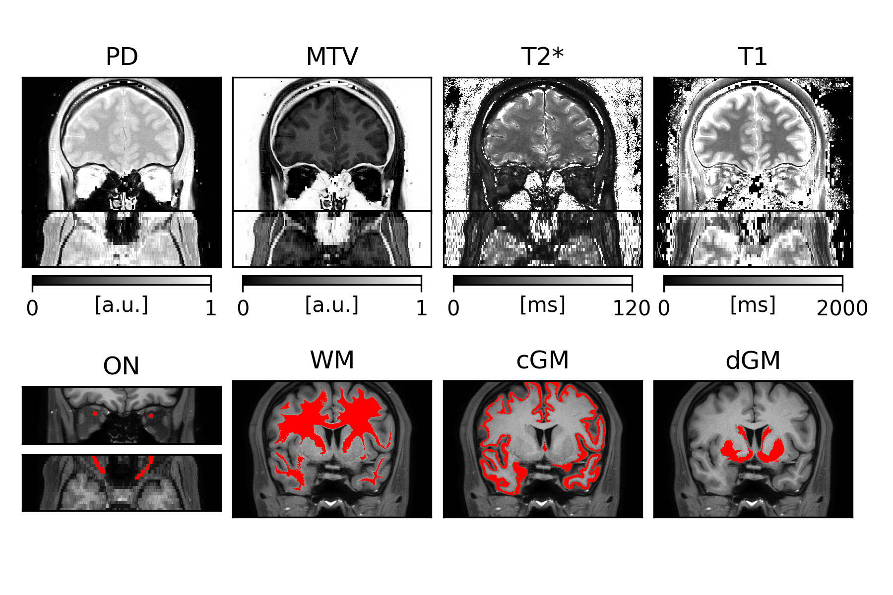
Figure 1. Examples of quantitative maps and regional masks for a single subject. Top row: PD, MTV, T2* and T1 quantitative maps coronal and axial slices. Bottom row: ON (coronal and axial slices), WM, cGM and dGM masks. The ON masks have been dilated for better visibility.
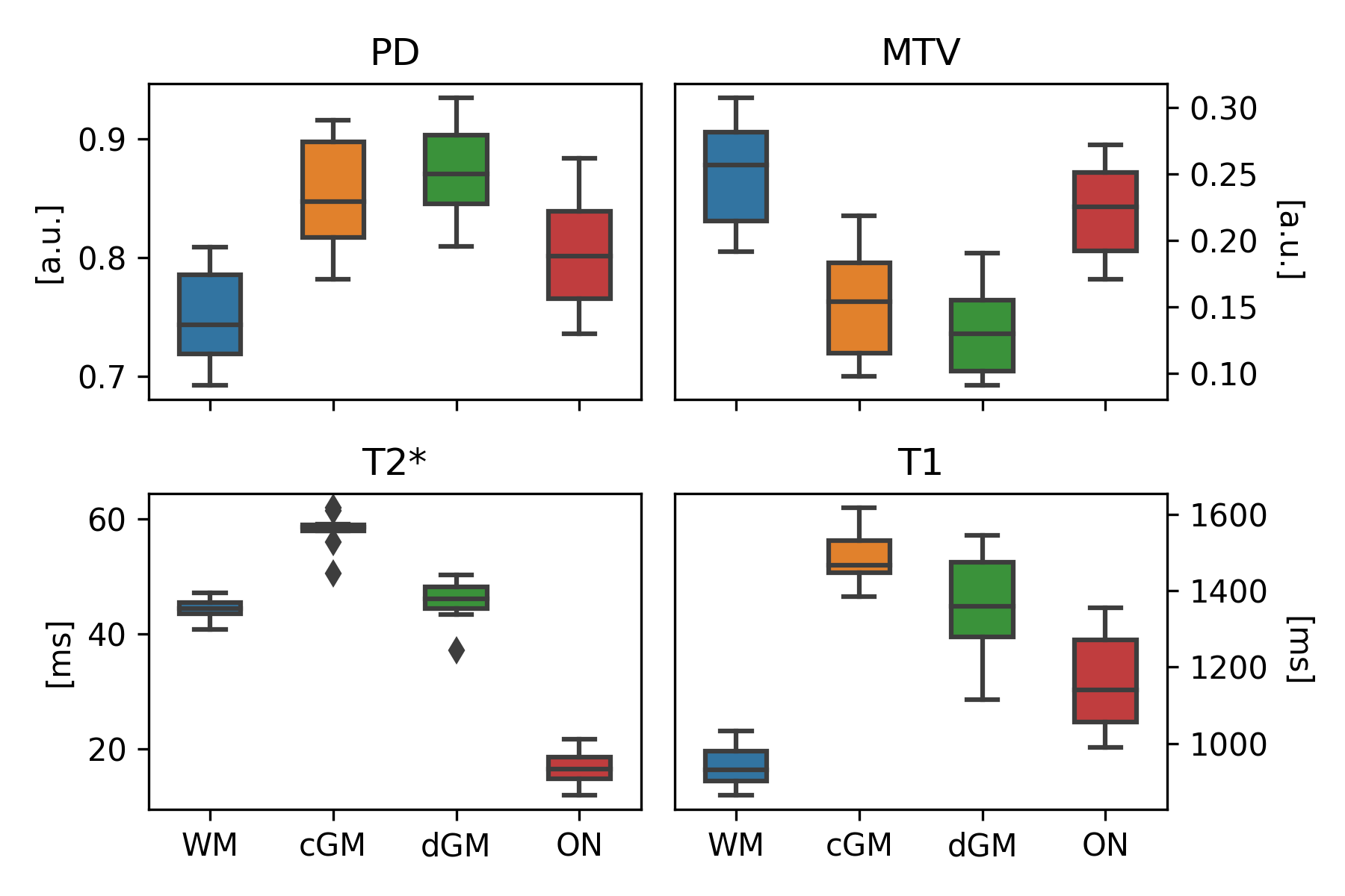
Figure 2. Distributions of regional values. For each quantitative MRI metrics, ON scores display a similar behaviour compared to brain tissues in terms of value distribution, whilst also exhibiting a specific range that makes them significantly different from white or grey matter.
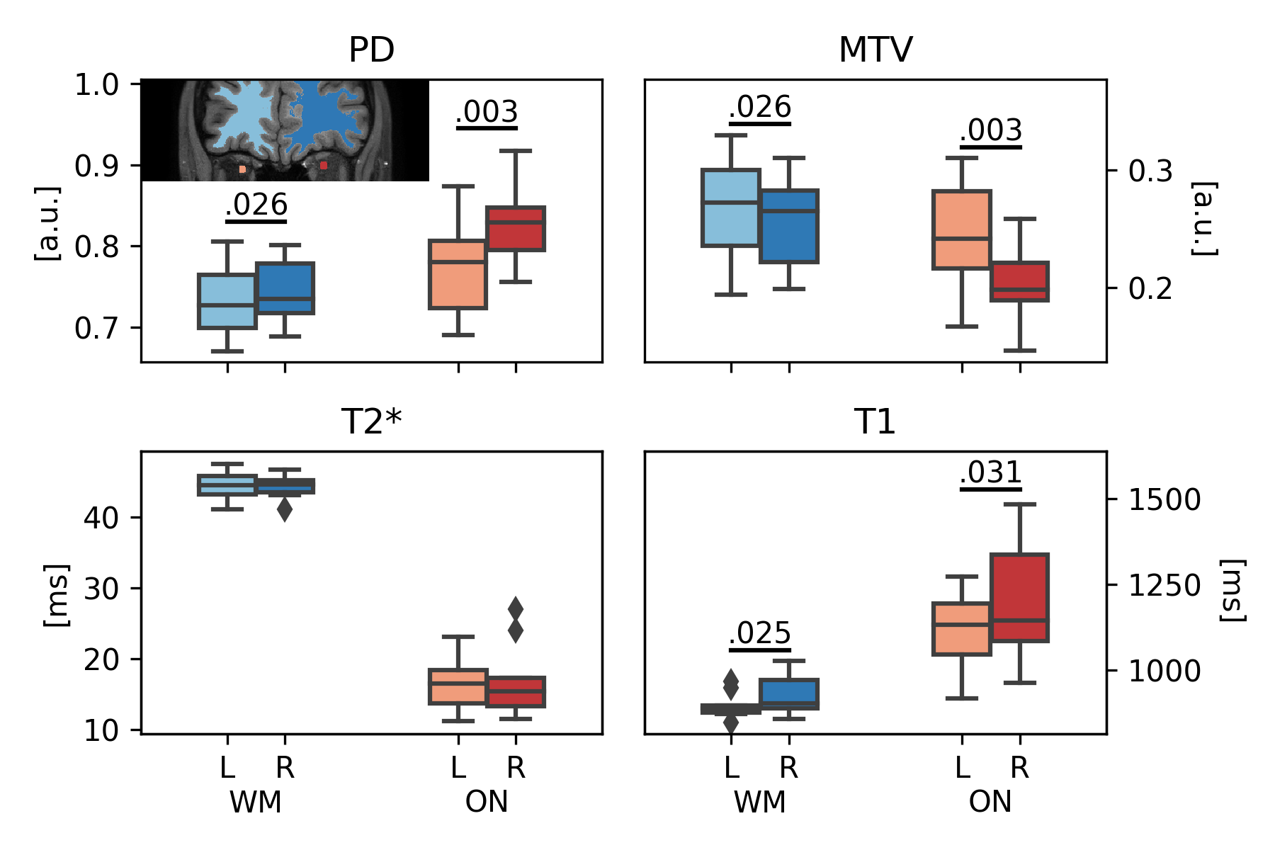
Figure 3. Laterality test. Significant differences were observed in PD, MTV and T1 between left (L) and right (R) ON and fronto-temporal WM (p-values reported). An example of left and right ON and fronto-temporal WM is displayed in the top-left corner.
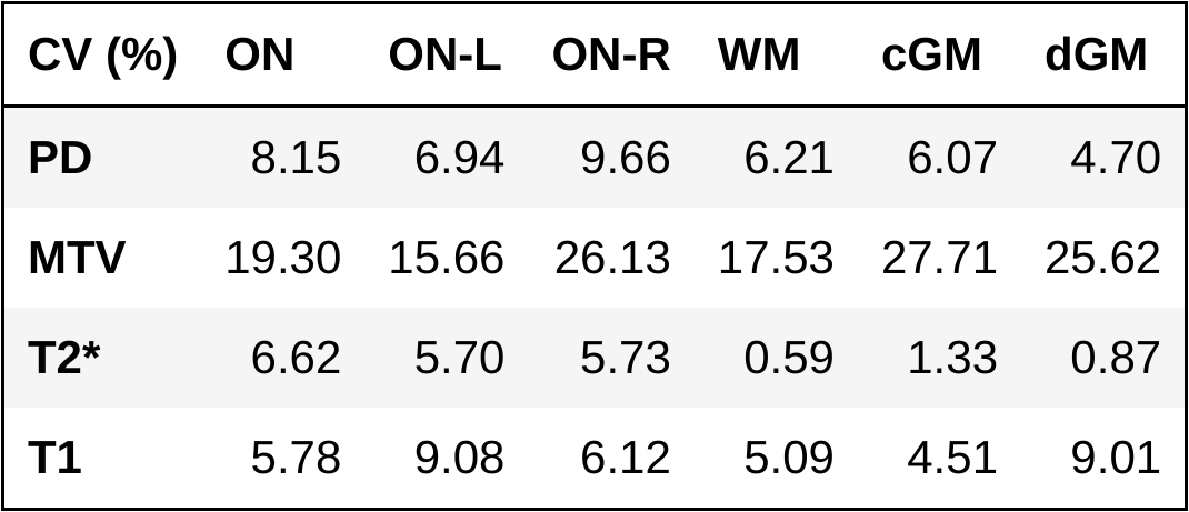
Table 1. Coefficients of variation for scan-rescan reproducibility. The higher MTV scores are due to MTV=1-PD inheriting variance from PD, whilst having lower mean.
DOI: https://doi.org/10.58530/2023/1190