Synopsis

Keywords: Quantitative Imaging, Brain Connectivity, Connectome, Histology, Phantom

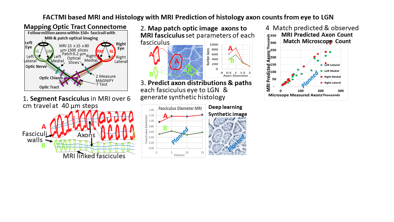
Accurate brain connectome mapping requires tracking fasciculus bundles of axons within tracts. In porcine optic nerve harvested tissue and TAXON diffusion phantom on a 14T magnet with a new linear coil array, we identify fasciculi with 16 µm resolution and follow TAXON fibers over centimeters from eye to LGN. MAGNIFY and bright field optical histology provide 0.1 & 0.25-micron resolution with accurate counts of the 1.2 million axons within fasciculi aligned with MRI and fasciculus wall structure. We use MRI and deep learning to predict the axon paths at each point and axon counts in each fasciculus.

Introduction

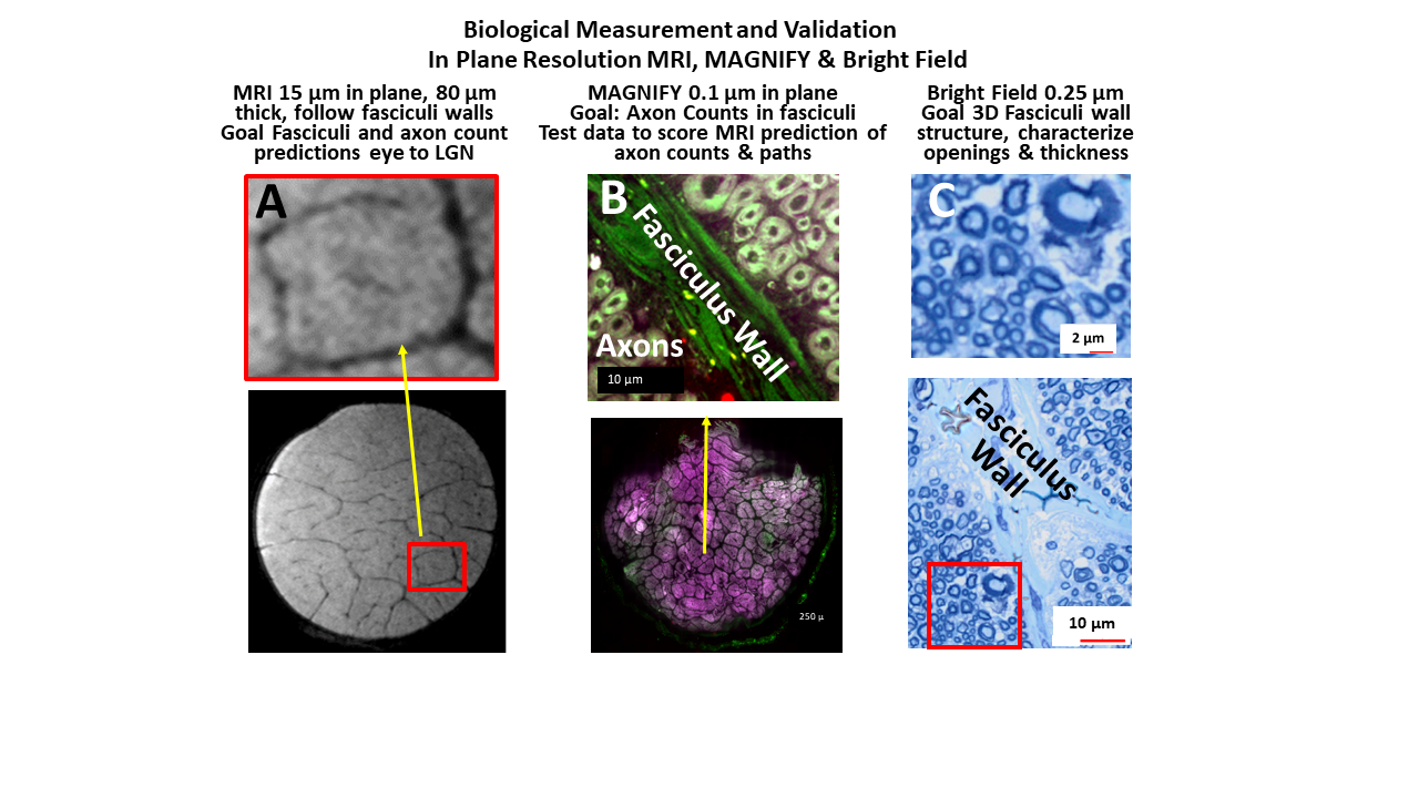
Accurate connectome tract mapping is yet an unachieved goal of imaging of our times. In MRI mapping, the estimated hit-false alarm has low accuracy (e.g, 13%[1] ). Histology can provide axon counts but not follow bundles of axons over centimeters of length. We are developing Fasciculus Axonal Connective Tissue Multiscale Imaging (FACTMI) technology to accurately map the over a million axon paths within 150+ fasciculi in the early optic system eye through chiasm to LGN. We follow the fasciculi walls with 16-micron MRI to quantify the axons in each fasciculus at nine slices along the path at viable cost in harvested porcine, rhesus, and human tissue. We provide ground truth phantom accuracy assessment and biological validation based on predicted axon counts of fasciculi within. Large mammals have fasciculi with connective tissue walls with a thickness of 20-80 microns. In FACTMI we follow the fasciculus walls with MRI. The axons at points along the tract can be quantified with histology slices post MRI. We follow fasciculi with 16x16x40 micron MRI from eye to LGN. This requires advanced approaches in MRI for 16-micron imaging with parallel micro coil arrays. The key test is whether we can predict the path and number of axons in fasciculus at every centimeter from the eye to LGN from MRI. We use MAGNIFY images to get axon counts in the early optic nerve and then predict the axon counts based on MRI at each of our nine test points along the optic nerve. We do axon counting with 0.1 micron optical imaging MAGNIFY[2] , and fasciculus wall mapping at 0.25 micron bright field optical imaging in 4-micron thick slices. Accuracy can be scored by comparing the predicted axon count for each fasciculus based on MRI imaging.

Methods

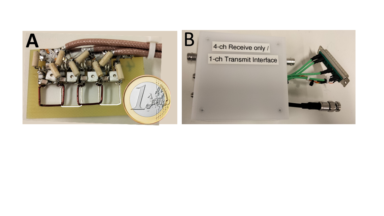
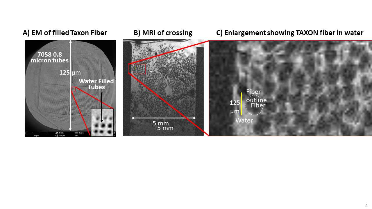
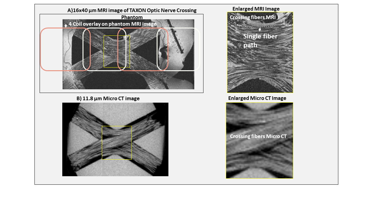
FACTMI involves multiple methods with differential strengths and costs to deliver full brain to 0.1 micron feature quantification. These methods require harvested tissue and work on large mammal tracts, including humans, rhesus, pigs, and rats that have tracts that are over 2 mm in diameter; mice optic nerve tracts are too small. MRI 16x16x40 micron full brain imaging with micro coil array at 14T of 5 mm harvested tissue slices and TAXON phantom. Figure 1 shows the receive coil array with four 10 mm coils in a linear line. Adjacent coil elements are geometrically decoupled and actively detuned during transmit via a 7.5 cm birdcage coil. The receive coil diameter was adjusted to cover about 10 mm in depth. The total sensitive area of the receiver array was about 10 mm x 37 mm. We used a TAXON[3] phantom and pig optic nerve tissue for scanning. The phantom images were acquired with a gradient echo sequence with resolution = 16 x 16 x 40 um, Matrix = 768 x 1024 x 512, FOV = 30.72 x 16.38 x 8.192 mm, TR = 50 ms, TE = 10.5 ms, alpha = 10°, Bandwidth 55555 Hz at 14.1 T within 14.5 hours. Figure 2 A shows MRI images of the optic nerve obtained with a spin echo sequence and a resolution of 20 x 20 x 80 um within 10 hours. For Optical Histology we used 0.1 micron MAGNIFY for axon counts within fasciculi (Figure 2B) and 0.25 micron bright field imaging (Figure 2C) for fasciculus wall structure. MAGNIFY[2] involves tissue expansion and labeling of myelin to show axons and connective tissue collegian to label fasciculus walls. This histology method images axon counts within each of the 150+ fasciculi in an optic nerve. The bright field imaging provides detailed picture of the fasciculus surface to characterize the fasciculi opening, merges, and splits. Phantom based ground truth imaging of 125 micron fibers with 7058 0.8 micron TAXON[3] tubes with 11.8 micron Micro CT that is compared to 16 micron MRI to follow fasciculi scale bundles of axon size tubes to score axon tracts. See Figure 5B. Following fasciculus walls with MRI eye to LGN can predict axon counts within fasciculi with MAGNIFY with 0.1 micron resolution to quantify axon diameters greater than 0.5-microns. See Figure 4.

Results

Figures 4 & 5 show fine detail of following the 125-micron fibers over centimeter distances in MRI with individual fibers identifiable generally with water surrounding them on the phantom. When viewing the slice stack, one can see fibers that cross or stay on the ipsilateral side migrating in the coronal slices in Figure 4B or in view in axial slices in Figure 5 A and B.

Discussion

The MRI resolution is sufficient to identify fasciculi walls with 16 x 16x 40-micron voxels in viable imaging time on a 14T magnet for harvested tissue. The linear coil allows parallel acquisition to reduce scanning time. We are planning to increase the array to 16 channels with custom-designed, CMOS-integrated transceiver electronics to collect MRI data on the full optic nerve in parallel. The methods work with histology (Figure 2) aligned assessment that can then be used in the prediction of axon counts with fasciculi that can be compared with the MAGNIFY axon counts (Figure 3).

References

1. Maier-Hein, K.H., et al., The challenge of mapping the human connectome based on diffusion tractography. Nature communications, 2017. 8(1): p. 1-13.
2. Klimas, B. Gallagher, P. Wijesekara, S. Fekir, D. Stolz, F. Cambi, S. Watkins, A. L. Barth, C. Moore, X. Ren, Y. Zhao*, “Nanoscale Imaging of Biomolecules using Molecule Anchorable Gel-enabled Nanoscale In-situ Fluorescence Microscopy”. Nature Biotechnology, accepted. Preprint available: Research Square; 2021. DOI: 10.21203/rs.3.rs-858006/v1.
3. Sudhir Pathak, Walter Schneider, Anthony Zuccolotto, Susie Huang, Qiuyun Fan, Thomas Witzel, Lawrence Wald, Els Fieremans, Michal E. Komlosh, Dan Benjamini, Alexandru V Avram, and Peter J. Basser Diffusion ground truth quantification of axon scale phantom: Limits of diffusion MRI on 7T, 3T and Connectome 1.0 ISMRM 2020