1181
Quantitative transport mapping (QTM) of the brain with simulated microvasculature model1Sibley School of Mechanical and Aerospace Engineering,, Cornell University, Ithaca, NY, United States, 2Department of Radiology, Weill Cornell Medicine, New York, NY, United States, 3Meinig School of Biomedical Engineering, Cornell University, Ithaca, NY, United States
Synopsis
Keywords: Quantitative Imaging, Arterial spin labelling
We compared the quantitative mappings on the simulated the brain arterial spin labeling images with artificial microvasculature structures and perfusion properties. The QTM method gives similar quantification on blood flow as the traditional tracer kinetic model.Introduction
Perfusion quantification models the tracer transport via temporal-sequence imaging. Traditional tracer kinetic model based on Kety equation1 with Tofts’ generalization2 links the temporal tracer concentration change to the arterial input function (AIF) for each voxel. However, as the AIF in each voxel is not measurable, the global AIF only considers temporal changes is applied in practice. This oversimplified assumption intrinsically causes errors in quantitative perfusion mapping3. Here we use quantitative transport mapping (QTM)4, an AIF-free method, to quantify perfusion mapping. We demonstrate that on the computational fluid dynamics (CFD) simulated brain microvascular structure, QTM method shows comparable ability on quantitative mapping as the traditional tracer kinetic model.Methods
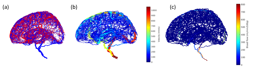
In the brain microvascular structure simulation, we used constrained constructive optimization5–7 method to generate the branches of the micro-vessels. The radius of mother and daughter vessels follows cubic rules: $$$r_M^3=r_{d1}^1+r_{d2}^1$$$. Meanwhile, unlike the common plug flow assumption8, we applied the quadratic blood velocity profile4 which is more realistic for pipe flow. Finally, the CFD simulated model was voxelized as arterial spin labeling (ASL) images.Both the traditional tracer kinetic method and QTM were implemented for quantification. The blood flow mapping is acquired by fitting the simulated ASL multiple delay data to the signal model4,9,10:
$$\lambda{d}M(t_i)=Q\cdot2\alpha{M_0}T_1'exp\left(-\frac{\delta}{T_{1b}}\right)\cdot\left[1-exp(-\frac{min(t_i-\delta,\tau)}{T_1'})\right]\cdot{exp\left(-\frac{max(0,t_i-\tau-\delta)}{T_1'}\right)}$$
Here, $$$\lambda=1$$$ is the tissue/blood partition coefficient for the simulated data, $$$dM(t_i)$$$ is the difference between tagged and control images at post-label delays $$$PLD=t_i$$$. $$$Q$$$ is the blood flow, $$$\alpha=1$$$ is the labeling efficiency for the simulated data and $$$M_0$$$ is the proton density-weighted image. $$$\frac{1}{T_1'}=\frac{1}{T_{1t}}+\frac{Q}{\lambda}$$$ and $$$T_{1t}=780/920ms$$$ for white matter and gray matter respectively. $$$\delta$$$ is the arterial transit time of blood from the labeling location to the brain, $$$T_{1b}=1350ms$$$ for blood and $$$\tau$$$ is the labeling time.
For QTM, the tracer concentration profile satisfies the transport equation
$$-\nabla\cdot{c(\pmb{r},t)}\pmb{u}(\pmb{r})=\partial_tc(\pmb{r},t)$$
Here $$$c(\pmb{r},t)$$$ is the tracer concentration with temporal and spatial distribution, $$$\pmb{u}(\pmb{r})$$$ is the velocity field, $$$\nabla$$$ is the gradient operator and $$$\partial_t$$$ is the derivative of time. The velocity could be solved as an optimization problem with L1 total variance regularization. We chose $$$\lambda=5\times10^{-7}$$$ as the regularization weight by L-curve method11. N is the total number of frames.
$$u=\underset{u}{\operatorname{argmin}}\sum_{t=1}^N||\partial_tc(\pmb{r},t)\pmb{u}\pmb(\pmb{r})||^2_2+\lambda||\nabla\pmb{u}\pmb(\pmb{r})||_1$$
Results
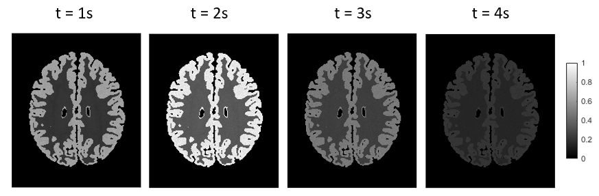
Figure 1 displays the simulated microvascular structure and the corresponding blood flow and velocity.Figure 2 exhibits the simulated ASL image frames with the normalized concentration. The concentration first increases and then decreases with the increase of time.
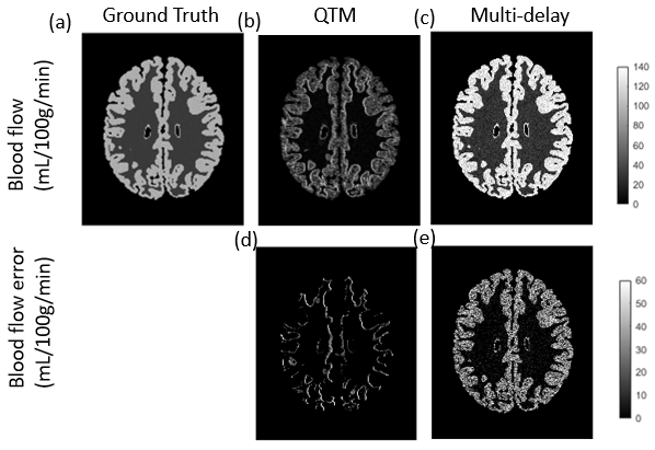
Figure 3a-c compares the ground truth voxelized blood flow with the quantitative results from the traditional kinetic model and QTM, respectively. Figure 3d-e show that QTM method gives generally similar blood flow error comparing to the traditional kinetic models.
Conclusion
We successfully demonstrate the functionality of the QTM method in perfusion quantification. The QTM method surpasses the traditional kinetic model on the CFD-simulated ASL data. The use of spatial concentration information contributes to accurate velocity mapping. A possible limitation of this work including the one-compartment model of QTM, which assume the impermeability of the vessels, and linear model estimation of tracer concentration, which is oversimplified in practice.Acknowledgements
No acknowledgement found.References
1. Kety, S. S. The theory and applications of the exchange of inert gas at the lungs and tissues. Pharmacol. Rev. 3, 1–41 (1951).
2. Tofts, P. S. et al. Estimating kinetic parameters from dynamic contrast-enhanced T(1)-weighted MRI of a diffusable tracer: standardized quantities and symbols. J. Magn. Reson. Imaging 10, 223–232 (1999).
3. Calamante, F. Arterial input function in perfusion MRI: a comprehensive review. Prog. Nucl. Magn. Reson. Spectrosc. 74, 1–32 (2013).
4. Zhou, L. et al. Quantitative transport mapping (QTM) of the kidney with an approximate microvascular network. Magn. Reson. Med. 85, 2247–2262 (2021).
5. Murray, C. D. The Physiological Principle of Minimum Work. Proceedings of the National Academy of Sciences 12, 207–214 (1926).
6. Neumann, F., Schreiner, W. & Neumann, M. Constrained constructive optimization of binary branching arterial tree models. https://www.witpress.com/Secure/elibrary/papers/OP95/OP95022FU.pdf.
7. Karch, R., Neumann, F., Neumann, M. & Schreiner, W. A three-dimensional model for arterial tree representation, generated by constrained constructive optimization. Comput. Biol. Med. 29, 19–38 (1999).
8. Buxton, R. B. et al. A general kinetic model for quantitative perfusion imaging with arterial spin labeling. Magn. Reson. Med. 40, 383–396 (1998).
9. Wang, D. J. J. et al. Multi-delay multi-parametric arterial spin-labeled perfusion MRI in acute ischemic stroke - Comparison with dynamic susceptibility contrast enhanced perfusion imaging. Neuroimage Clin 3, 1–7 (2013).
10. Dai, W., Robson, P. M., Shankaranarayanan, A. & Alsop, D. C. Reduced resolution transit delay prescan for quantitative continuous arterial spin labeling perfusion imaging. Magn. Reson. Med. 67, 1252–1265 (2012).
11. Calvetti, D., Morigi, S., Reichel, L. & Sgallari, F. Tikhonov regularization and the L-curve for large discrete ill-posed problems. J. Comput. Appl. Math. 123, 423–446 (2000).
Figures