Synopsis

Keywords: Signal Modeling, Velocity & Flow, time-of-flight, flow-enhanced fMRI signal

Fast fMRI has recently been shown to be an effective method for detecting dynamic changes in cerebrospinal fluid flow, enabling measurement of a critical process for maintenance of brain health. However, while the inflow signal measured using fast fMRI is a surrogate for the underlying flow dynamics, it does not directly reflect the velocity and dynamics of flow. To understand the mapping between flow and the flow-enhanced MR signals they generate, we developed and validated a mathematical forward model that uses velocity as input and simulates dynamic fMRI inflow signal intensities for each slice of the imaging volume.

Introduction

The flow of cerebrospinal fluid (CSF) is essential for maintenance of brain homeostasis, but the dynamics of CSF flow in the human brain remain poorly understood, in part due to technical challenges in flow measurements. A common method for quantifying fluid flow with MRI is phase contrast imaging. Fast fMRI has recently been shown to also be an effective method for detecting CSF flow ¹, by leveraging the well-known Time-of-Flight effect ², where inflow of fresh fluid generates bright signals. Measuring inflow signals with fMRI has several advantages: it can measure flow simultaneously with whole-brain blood-oxygenation-level-dependent (BOLD) signals; it has higher sensitivity to slow velocities than phase contrast imaging, making it well-suited to CSF flow; and it provides high temporal resolution. However, the disadvantage of the fMRI inflow signal is that it is not quantitative. The inflow signal is not directly proportional to velocity, and the mapping between flow speed and the inflow signal is nonlinear. To improve interpretation of dynamic inflow signals in fMRI, we developed and validated a model which takes a velocity timeseries as input, and simulates flow-enhanced fMRI signals. This approach can allow for quantification of fluid flow using fMRI, increasing information gained from neuroimaging studies.

Methods

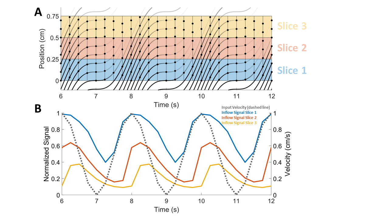
We developed a model to simulate the fMRI signals generated by fluid flow. The flowing media is discretized into protons separated by distance dx, with position X(t) defined by the integral of an input velocity V(t). Protons flow through imaging slices and receive RF pulses based on slice-specific timings (Fig.1A). The transverse magnetization (M_T) of protons depends on how many pulses it’s received (n) and the time between pulses (Δt):

$$$M_T=M_0\cos{\theta}\sum_{m=0}^{n-1}[\cos{\theta}^m(\prod\limits_{k=n-m}^{n-1}{e^{-\Delta{t_k/T_1}}})(1-e^{-\Delta{t_{n-m-1}}/T_1})]\sin{\theta}e^{-TE/T_2}\,\,\,\,n\ge1$$$ (Eqn.1)

where T₁ is the longitudinal relaxation time constant, θ is the flip angle, M₀ is the equilibrium longitudinal magnetization, TE is the echo time, and T₂ is the transverse relaxation time constant. We model flow-enhanced signals from individual protons as the difference between M_T and the steady state ($$$n\rightarrow\infty$$$ in Eqn.1), and to simulate timeseries of slice signal intensities, we average contributions from protons after each volume acquisition. When velocity increases, protons move faster through imaging slices and accumulate fewer RF pulses within each slice. When velocity is slow, protons spend more time in slices and their signals decrease (Fig.1).

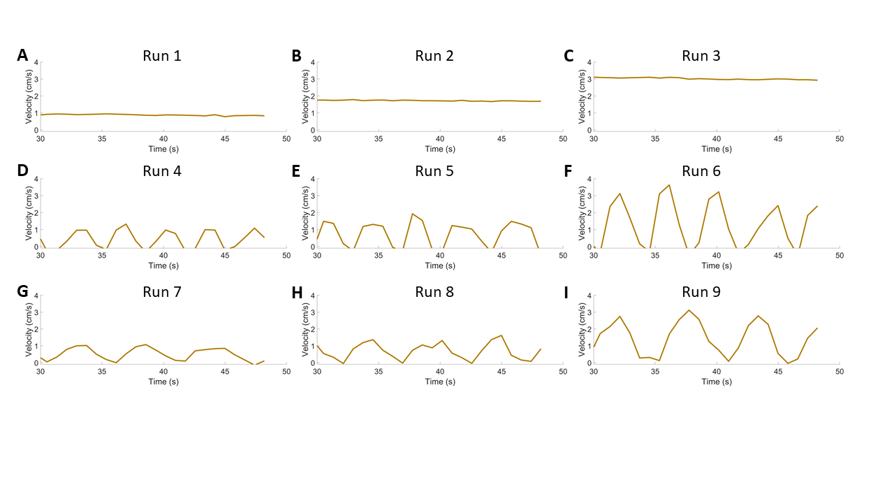
Validation experiments were conducted on a flow phantom and human, to assess how accurately the model can predict velocities from inflow-enhanced signals. The flow phantom consisted of a peristaltic pump connected to plastic tubes and a flow meter with adjustable velocity. The plastic tube was wrapped around an agar gel phantom and scanned on a 3T Siemens Prisma scanner. Each run was acquired during constant or oscillatory flow (Fig.2). For each flow condition, we performed a phase contrast scan (VENC=8cm/s, 3mm isotropic, TR=803ms, TE=6.7ms), followed by a BOLD fMRI scan (2.5mm isotropic, TR=340ms, TE=30ms, FA=37°).

A human participant was scanned on a 3T Siemens Prisma scanner. We first acquired an anatomical MPRAGE and used it to position imaging slices at the 4^th ventricle where CSF flow has been observed ³. To drive CSF pulsations, the subject performed 5 minutes of paced breathing with 6-second breath cycles ⁴. We performed 2 runs of phase contrast (VENC=8cm/s, 3mm isotropic, TR=803ms, TE=6.7ms), and 2 runs of BOLD fMRI (2.5mm isotropic, Multiband factor=3, TR=504ms, TE=30ms, FA=45°). We manually identified an ROI in the fourth ventricle and extracted its timeseries.

Results

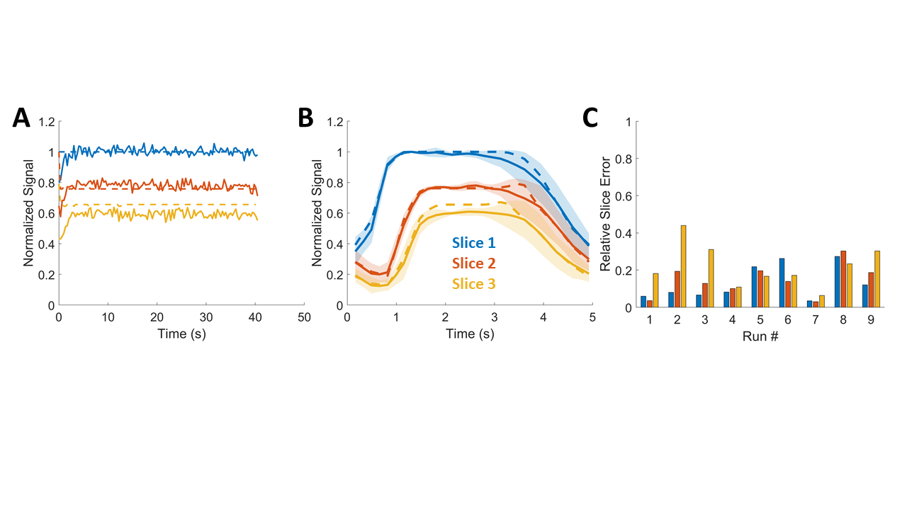
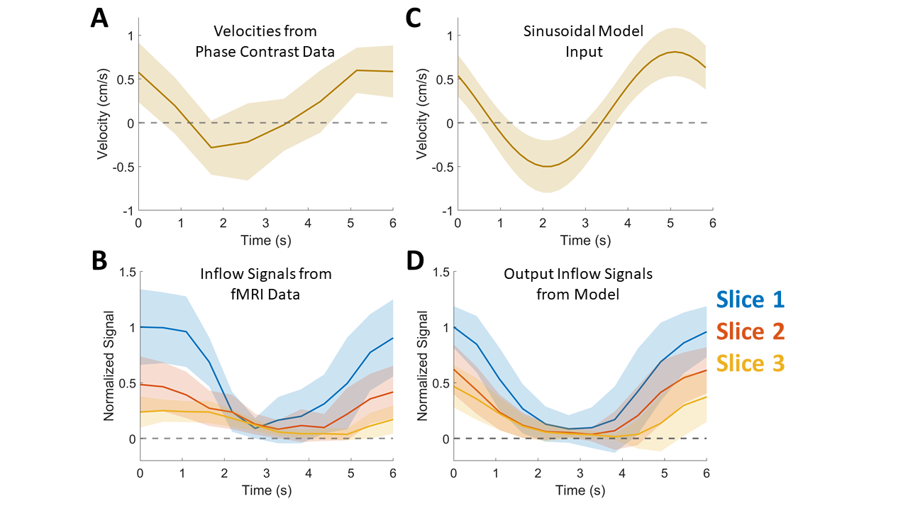
We first measured fMRI signals during constant flow in the phantom, and found that the model successfully predicted the relative slice signal amplitudes in the fMRI data (Fig.3A). A representative example from a time-varying input velocity shows that the model also captured the relative amplitudes of slice signals during oscillatory flow, and distinct timings at which signals rise and fall (Fig.3B). We assessed model performance by using phase contrast velocities as input and calculating the relative errors between simulated inflow signals and measured inflow signals, for each slice. Overall, the model closely matched data over a range of input conditions, with a tendency to be more accurate for slower flows (Fig.3C). We next tested the model in the human imaging data, where CSF flow is always pulsatile. We identified the distribution of respiratory-locked CSF flow using the phase contrast data (Fig.4A): for each cycle of respiratory-locked CSF flow, we measured minimum and maximum velocities, and used a sinusoid with that minimum and maximum velocity as model input (Fig. 4C). The dynamics and amplitudes of the resulting simulated slice signals (Fig.4D) closely matched the fMRI slice-dependent data during paced breathing (Fig. 4B). These results demonstrated successful prediction of the fMRI signals induced by a range of CSF velocities, in human data.

Discussion

Here, we developed and validated a mathematical model that simulates dynamic fMRI inflow signals caused by a given flow velocity. Results demonstrated that the model can predict the velocities of the fluid that generates inflow-enhanced fMRI signals, and this method could be used to test which fluid velocity could produce an observed fMRI signal. This work enables future neuroimaging studies to simultaneously monitor hemodynamics and quantitative changes in the speed and dynamics of fluid flow such as CSF.

References

1. Fultz, N. E., Bonmassar, G., Setsompop, K., Stickgold, R. A., Rosen, B. R., Polimeni, J. R., & Lewis, L. D. (2019). Coupled electrophysiological, hemodynamic, and cerebrospinal fluid oscillations in human sleep. Science, 366(6465), 628-631.
2. Gao, J. H., Miller, I., Lai, S., Xiong, J., & Fox, P. T. (1996). Quantitative assessment of blood inflow effects in functional MRI signals. Magnetic resonance in medicine, 36(2), 314-319.
3. Chen, L., Beckett, A., Verma, A., & Feinberg, D. A. (2015). Dynamics of respiratory and cardiac CSF motion revealed with real-time simultaneous multi-slice EPI velocity phase contrast imaging. Neuroimage, 122, 281-287.
4. Dreha-Kulaczewski, S., Joseph, A. A., Merboldt, K. D., Ludwig, H. C., Gärtner, J., & Frahm, J. (2017). Identification of the upward movement of human CSF in vivo and its relation to the brain venous system. Journal of Neuroscience, 37(9), 2395-2402.