1168

Feasibility of automatic patient-specific sequence optimization with deep reinforcement learning

Maarten Terpstra^1,2, Sjors Verschuren^1,2, Tom Bruijnen^1,2, Matteo Maspero^1,2, and Cornelis van den Berg^1,2
¹Department of Radiotherapy, University Medical Center Utrecht, Utrecht, Netherlands, ²Computational Imaging Group for MR Diagnostics & Therapy, University Medical Center Utrecht, Utrecht, Netherlands

Synopsis

Keywords: Pulse Sequence Design, Machine Learning/Artificial Intelligence, Autonomous sequence optimization

Introduction

For MRI-guided interventions, tumor contrast and visibility are crucial. However, the tumor tissue parameters can significantly vary among subjects, with a range of T1, T2, and proton density values[1] that may cause sub-optimal image quality when scanning with population-optimized protocols[1,2]. Patient-specific pulse sequence parameter optimization could significantly increase image quality, but manual parameter optimization is infeasible due to the vast number of parameters. One way to perform automatic patient-specific protocol optimization is by applying deep learning. Specifically, deep reinforcement learning (DRL) has been proposed as a fast and quickly-converging method for iterative optimization[3]. Here, we explore whether DRL can perform automatic patient-specific sequence optimization with minimal additional scan time. As a proof of concept, DRL was used to optimize the flip angle of steady-state spoiled gradient echo (SPGR) acquisitions.

Materials and methods

Two DRL models were trained on synthetic data: one to maximize the signal-to-noise ratio (SNR) and one to maximize the contrast-to-noise ratio (CNR). The models were implemented in an automatic feedback loop with the MRI (Fig. 1). The trained models were applied to phantoms to maximize the SNR and CNR automatically and in-vivo to maximize the CNR in manually-delineated regions-of-interest (ROIs).

Training & model architecture
The signal from SPGR acquisition of isochromats from random tissue with a uniform distribution of T1 and T2 values (T1$$$\in$$$[100-2000]ms, T2$$$\in$$$[25-150]ms, TR=10ms) and a random initial flip angle value $$$\alpha_{\text{init}} (\alpha\in[5-50])$$$ was simulated using the extended phase graph method[4]. We used the recurrent deterministic policy gradient (RDPG) architecture[5] to maximize the SNR and CNR between two isochromats. The RDPG architecture uses recurrent actor-critic neural networks. The actor learns, given an observation o_t, the flip angle $$$\alpha_{t+1}$$$ that maximizes future rewards and the critic estimates the future reward of an action $$$\mathbf{a}_t$$$ given o_t (Fig. 2). Recurrent information ensures that previously-optimized scans are considered, enabling fast and stable convergence of the parameters. Two different RDGP models were trained: one to maximize the SNR in a single isochromat and one to optimize the CNR between two isochromats. The reward was computed as the relative SNR/CNR improvement $$$(M_{t+1}-M_t)/M_t$$$, where $$$M$$$ is the SNR or CNR, respectively. The new flip angle was computed as $$$\alpha_{t+1}=\alpha_t\cdot(\mathbf{a}_t+1)\text{ if }\mathbf{a}_t\geq0\text{ else }\alpha_t\cdot(\mathbf{a}_t/2+1),\mathbf{a}_t\in[-1,1]$$$. The model was trained to optimize an episode, i.e., a sequence of $$$T$$$ consecutive ($$$o_t,\mathbf{a}_t$$$) steps. The model was trained using 10000 episodes of $$$T$$$=10 timesteps $$$t$$$, with a batch size of 64 and was optimized using truncated backpropagation-through-time[6] of five timesteps with the Adam optimizer. Gaussian random noise (N(0,1)) was added to the models' chosen actions to ensure the exploration of the action space.

Experiments & Implementation
RabbitMQ was used to establish autonomous, bi-directional communication between a 1.5T MRI-Linac (Philips Healthcare, Best, the Netherlands) and the DRL agent, enabling the transfer of observations $$$o_t$$$ and the updated flip angle $$$\alpha_{t+1}$$$. Two phantoms were scanned: a water bottle where the SNR was maximized within a manually-delineated ROI and a phantom with different T1, T2, and PD tubes to maximize the CNR between the two tubes. All scans were acquired using a 2D-SPGR acquisition (TE/TR = 25/50 ms) with a random initial flip angle. The experiments were repeated for ten different random $$$\alpha_{\text{init}}$$$ to measure the average performance. Moreover, the SNR and CNR of the phantoms were measured for all $$$\alpha\in[1,2,3,\ldots,50]$$$ (Fig. 3). The pelvis of a healthy volunteer was scanned to maximize the CNR between ROIs in the gluteus maximus and nearby fatty tissue. The Ernst angles giving optimal SNR/CNR were analytically computed for the phantoms and empirically established in-vivo.

Results

Acquisition and reconstruction took approximately 2 seconds, and the subsequent communication overhead and model inference took about one second. In the example of the feedback loops reported in Fig. 3, the model significantly increased the SNR and CNR in the phantom scans achieving 99% and 97% of the optimal SNR and CNR in five steps, respectively. On average, over the ten repeated scans, the model reaches 98.8±1.3% ($$$\mu\pm\sigma$$$) of the optimal SNR and 96.8±1.6% of the optimal CNR within five scans and shows stable convergence (Fig. 4). For the in-vivo results, the model maximized the CNR between muscle and fat tissue achieving 96% of the optimal CNR within four additional acquisitions (Fig. 5).

Discussion & Conclusion

We have implemented a patient-specific sequence optimization framework using a DRL agent to quickly maximize the SNR and CNR for phantom and in-vivo acquisitions. The model achieved near-optimal SNR/CNR in five additional acquisitions (about 10 seconds). We consider this additional scan time acceptable but might prove too long for 3D acquisitions. However, the extra scan time could be minimized by designing efficient surrogate examinations (e.g., using low image resolution). With this proof-of-concept we demonstrated that DRL can optimize pulse sequence parameters automatically in an in-vivo scenario, even when trained on simulated data. Future work will investigate extending the model to optimize for multiple parameters simultaneously, e.g., TE, TR, or RF pulse shape, which is a more complex optimization problem but could lead to even higher image quality and contrast[7,8,9]. We demonstrated that DRL could be used for subject-specific contrast optimization with a minimal additional scan time. In the future, DRL-based sequence optimization could facilitate MRI-guided interventions by optimizing tumor contrast.

Acknowledgements

This work is part of the SIGNET project, which is a project in the ITEA program. We gratefully acknowledge the support of NVIDIA Corporation with the donation of the Quadro RTX 5000 GPU used for prototyping this research.

References

[1] Navest et al. (2022). Personalized MRI contrast for treatment guidance on an MRI-linac in patients with liver metastases. Proc. ESTRO

[2] Gabr et al. (2016). Automated patient‐specific optimization of three‐dimensional double‐inversion recovery magnetic resonance imaging. MRM, 75(2), 585-593.

[3] Zhou et al. "Deep reinforcement learning in medical imaging: A literature review." Medical image analysis 73 (2021): 102193.

[4] Weigel, M. (2015). Extended phase graphs: dephasing, RF pulses, and echoes‐pure and simple. Journal of Magnetic Resonance Imaging, 41(2), 266-295.

[5] Heess et al. (2015). Memory-based control with recurrent neural networks

[6] Williams, R. and Peng, J. (1990). An efficient gradient-based algorithm for on-line training of recurrent network trajectories. Neural Computation, 2(4):490–501.

[7] Zhu et al. (2018). AUTOmated pulse SEQuence generation (AUTOSEQ) using Bayesian reinforcement learning in an MRI physics simulation environment. Proc. Int Soc. Mag. Res. Med.

[8] Loktyushin et al. (2021) MRzero - Automated discovery of MRI sequences using supervised learning. MRM

[9] Glang et al (2022) MR-double-zero – Proof-of-concept for a framework to autonomously discover MRI contrasts. JMR

Figures

Figure 1: Overview of the feedback loop. The recurrent deep reinforcement learning (RDPG) agent performs patient-specific pulse sequence optimization in a real-time feedback loop. The model iteratively updates the sequence parameters to improve the SNR and CNR per-patient having as input the acquired MRI. Bi-directional communication of the acquired MRI and new sequence parameters was performed using a RabbitMQ message queue with a cycle time of about three seconds for a 2D acquisition.

Figure 2: Deep reinforcement learning model architecture. The RDPG architecture consists of two models: an actor and a critic, which share the same architecture. The actor proposes an action a_t ∈ [-1,1] that maximizes the future reward $$$\hat{Q}$$$(o_t,a_t), as calculated by the critic. The critic learns the true future reward Q(o_t,a_t). The model consists of a fully-connected (FC) layer (yellow) of 64 units with ReLU activation, two LSTM layers (red), and an FC layer mapping to the output. The actor uses a final TanH activation to limit the output to ±1. The models used up to T=10 timesteps.

Figure 3: Performance characteristics (animation). On the left are examples of optimizations performed by the RDPG. The first image is the initial image, and the RDPG optimized every subsequent image. The blue points are the SNR and CNR of the optimized images, and the red dot is the current image. On the right, the SNR and CNR for every flip angle between 1 and 50 degrees. The SNR of the phantom is optimal at a flip angle of 14 degrees, while the CNR between the highlighted tubes is maximal at a flip angle of 23 degrees. The model reached 97% of the optimal SNR and CNR within five subsequent scans.

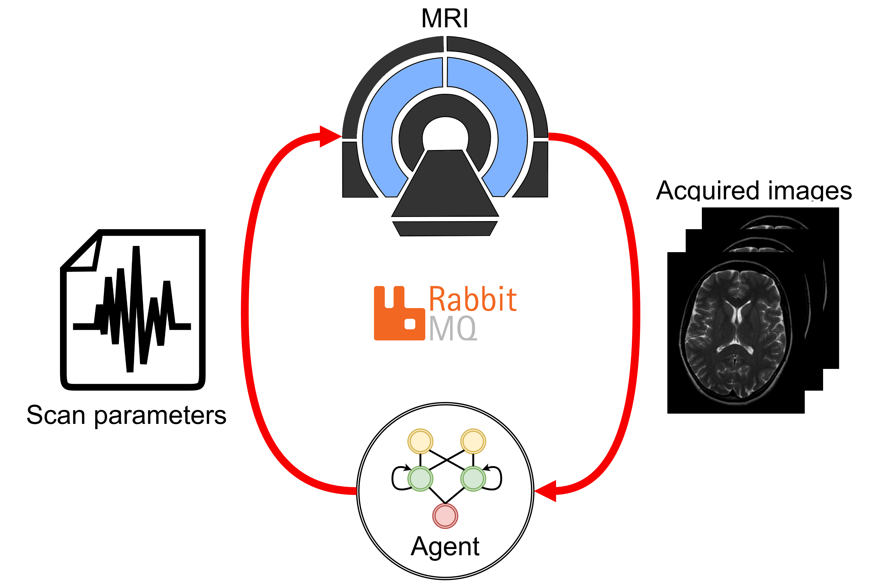
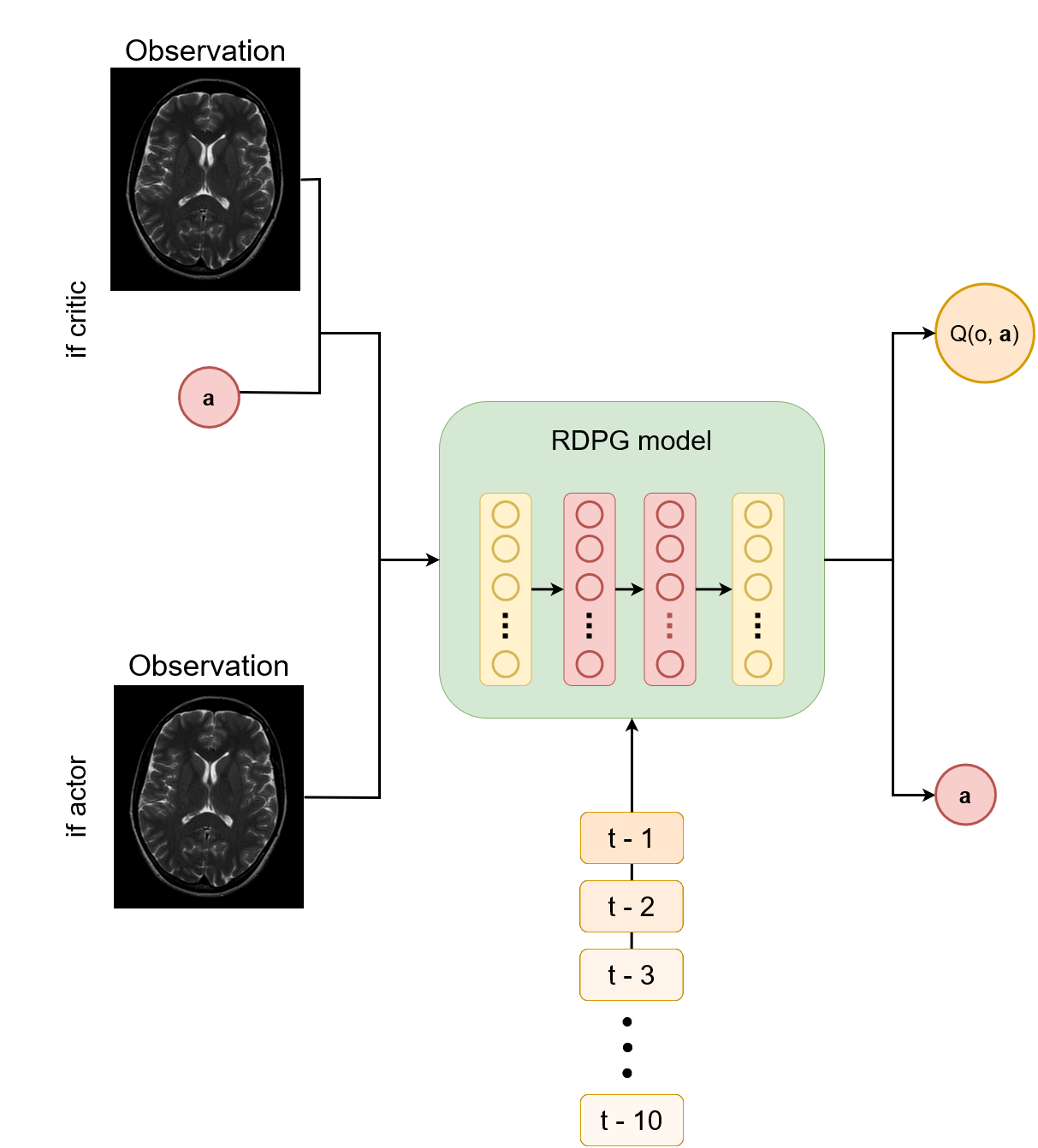
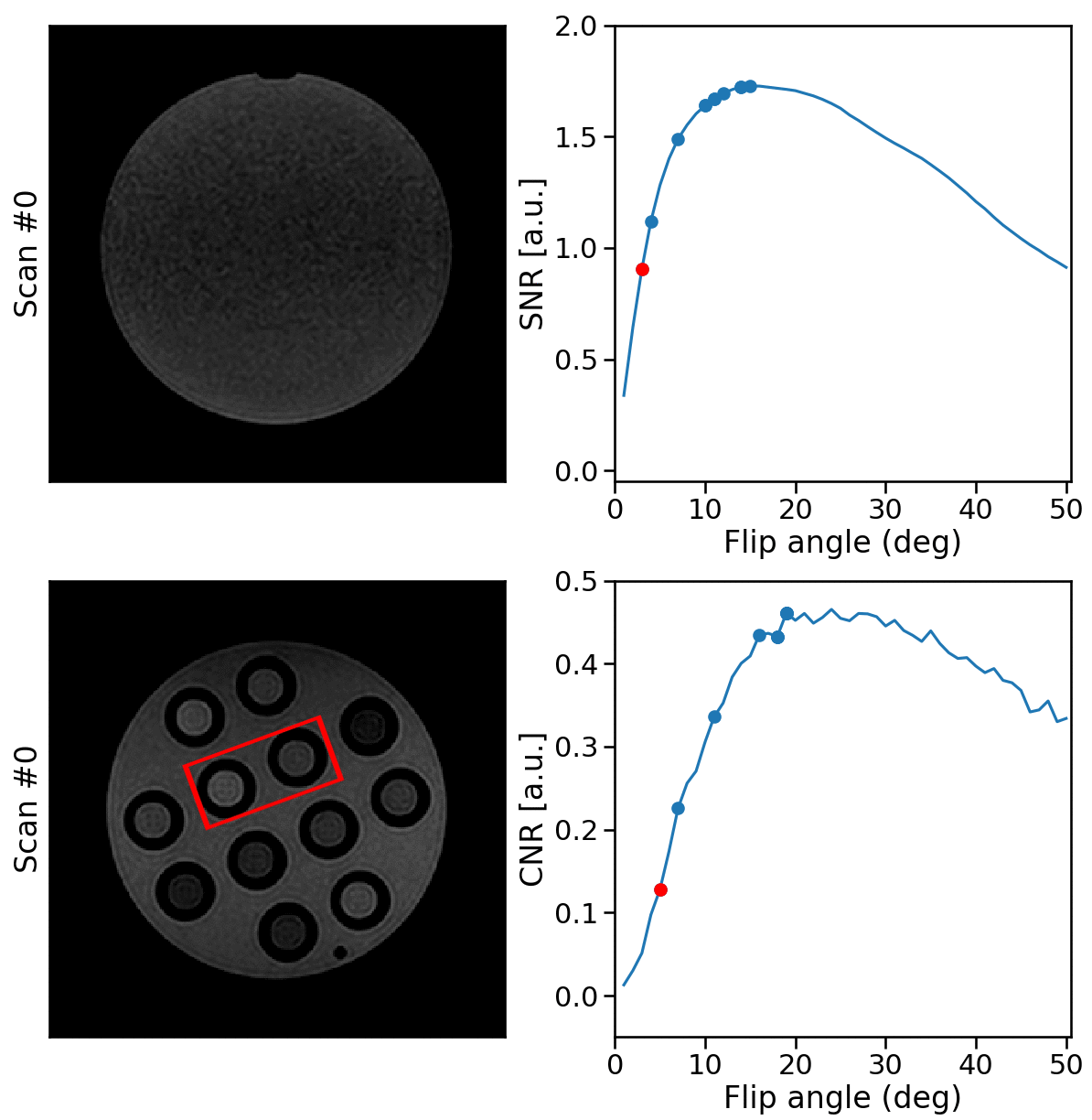
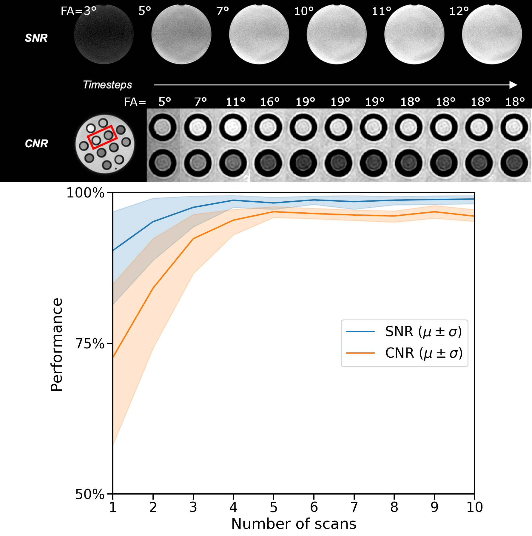
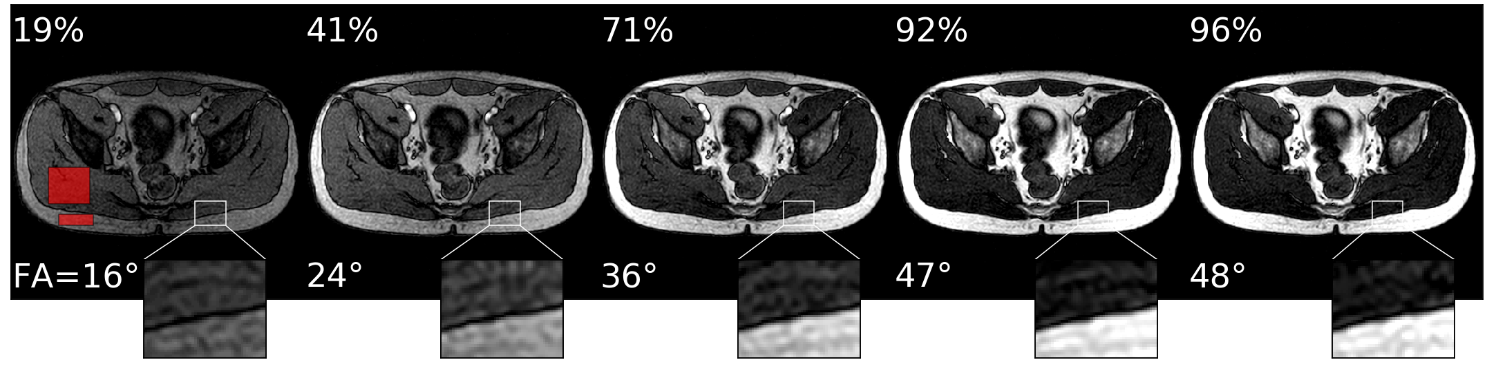
Figure 4: phantom results. The top rows show examples of phantom SNR and CNR optimizations with corresponding flip angles. The first image is the initial image, and the RDPG model optimized the following images. The SNR was computed within the phantom, and the CNR between the highlighted tubes. After five steps, the model reached 99% and 97% of the optimal SNR and CNR, respectively. The bottom graph shows the quantitative results for ten different initial flip angles α_init. Within ten additional scans, the model converges near the optimal SNR/CNR regardless of the initial flip angle.

Figure 5: In-vivo results. The CNR was maximized between the red rectangles in an online in-vivo setting. The top number is the relative CNR compared to the optimal CNR, as empirically determined at 50 degrees. The bottom number shows the flip angle, while the zoomed region highlights the contrast. The first scan is the starting image, and within four steps, the model reaches 96% of the optimal CNR. The acquisition time per image was approximately two seconds, while data communication and model inference took about 1 second.

Proc. Intl. Soc. Mag. Reson. Med. 31 (2023)

1168

DOI: https://doi.org/10.58530/2023/1168