1166

Semi-Supervised Learning for Spatially Regularized Quantitative MRI Reconstruction - Application to Simultaneous T₁, B₀, B₁ Mapping

Felix Frederik Zimmermann¹, Andreas Kofler¹, Christoph Kolbitsch¹, and Patrick Schuenke¹
¹Physikalisch-Technische Bundesanstalt (PTB), Berlin and Braunschweig, Germany

Synopsis

Keywords: Quantitative Imaging, Machine Learning/Artificial Intelligence

Typically, in quantitative MRI, an inverse problem of finding parameter maps from magnitude images has to be solved. Neural networks can be applied to replace non-linear regression models and implicitly learn a suitable spatial regularization. However, labeled training data is often limited. Thus, we propose a combination of training on synthetic data and on unlabeled in-vivo data utilizing pseudo-labels and a Noise2Self-inspired technique. We present a convolutional neural network trained to predict T₁, B₀, and B₁ maps and their estimated aleatoric uncertainties from a single WASABITI scan.

Introduction

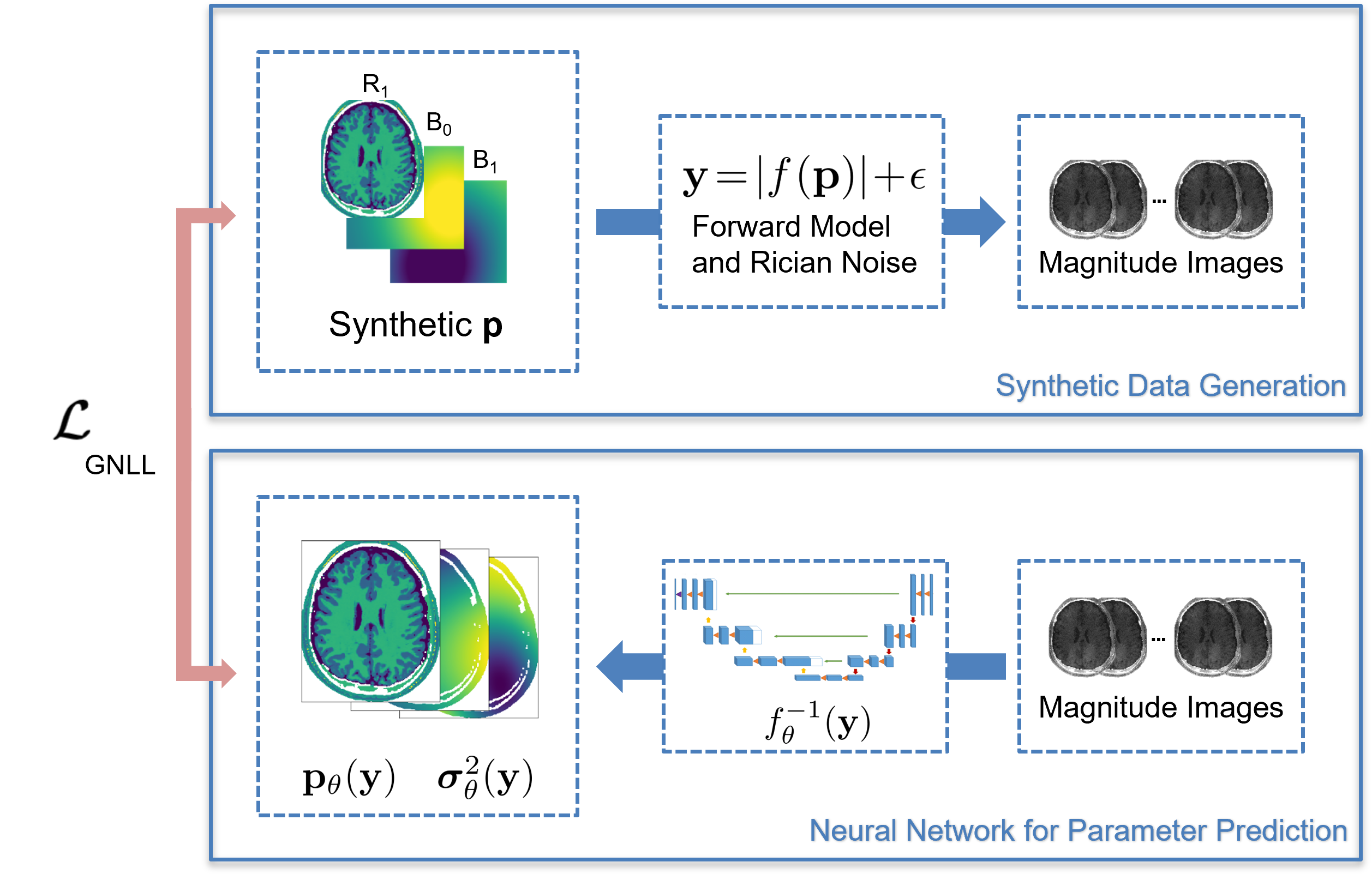
Quantitative MRI applications most of the time require solving inverse problems
$$\mathbf{y}=\left| f(\mathbf{p})\right|+\mathbf{\epsilon}$$ where $$$\mathbf{p}$$$ denotes a vector of quantitative parameters (e.g. relaxation times and field inhomogeneities), $$$\mathbf{y}$$$ a series of magnitude images, $$$\mathbf{e}$$$ Rician noise and $$$f$$$ the non-linear signal model. A solution can either be found by a (non-linear) regression^1,2 or by deep learning approaches^3-7. Noise in the data can strongly impair the accuracy of these approaches. This can be overcome with spatial regularisation which improves the conditioning of this ill-posed problem. To ensure fast and robust quantitative MRI, we combine deep learning-based parameter estimation and learning spatial regularisation by using a convolutional neural network (CNN) approach. We apply this to WASABITI^1,3, a method that allows predicting $$$\mathbf{p}=\left[T_1;B_0;B_1\right]$$$ from a single CEST-like scan. As acquiring enough WASABITI measurements with ground truth labels for the parameter maps by reference methods would be infeasible, we propose a combination of training on synthetic data and unsupervised fine-tuning on label-free in-vivo measurements.

Methods

We used the well-known U-Net architecture⁸ with 4 layers, 32 initial filters, and roughly 5 million parameters to predict T₁, B₀, B_1, and aleatoric uncertainties from normalized measurements of WASABITI. We generated synthetic relaxation time maps based on the Brainweb⁹ dataset of segmented brains by sampling T₁ for each tissue class. Synthetic B₀ and B₁maps were generated as a mixture of random 2D polynomials (3^rdorder) and randomly positioned 2D-Gaussians. From these maps, the simulated WASABITI data to be used as network input was generated by applying the analytical forward model based on the solution of the Bloch equations for off-resonance excitation¹⁰ and applying Rician noise with SNR randomly chosen from 3-30. Training was performed on a single GPU with AdamW optimizer, 10^-4 weight decay, 2*10^-4 maximum learning rate with a cosine schedule with warmup.

For fine-tuning on in-vivo data to learn a more realistic spatial regularization, we acquired data of 10 healthy volunteers. The measurements were performed on a 3T whole-body MRI scanner. The 31-point WASABITI sequence with 2D centric-reordered GRE readout sequence was implemented using the pulseq¹¹ framework. We split the data 9/1 for training/validation.

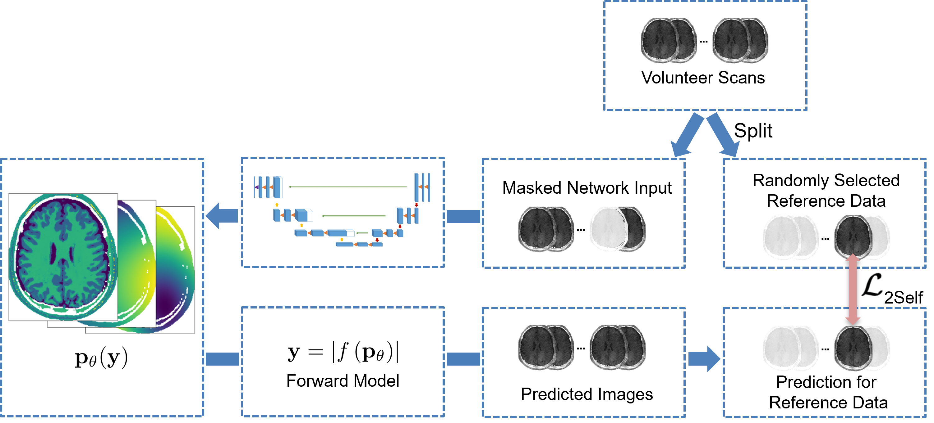
We used a modification of the Noise2Self¹² learning approach, similar to SSDU¹³: In each pixel of the inputs to the network, we mask out randomly one of the 31 measurement points (figure 3). Only these points are then used to calculate the L₂-loss $$$L_\textrm{2Self}$$$ after applying the forward model to the predicted parameters. Under the assumption, that the noise in different points of the spectra is uncorrelated, the optimal solution for the network will be to output the parameters resulting in the (unknown) noise-free measurement at the test points, thus avoiding fitting to the noise.

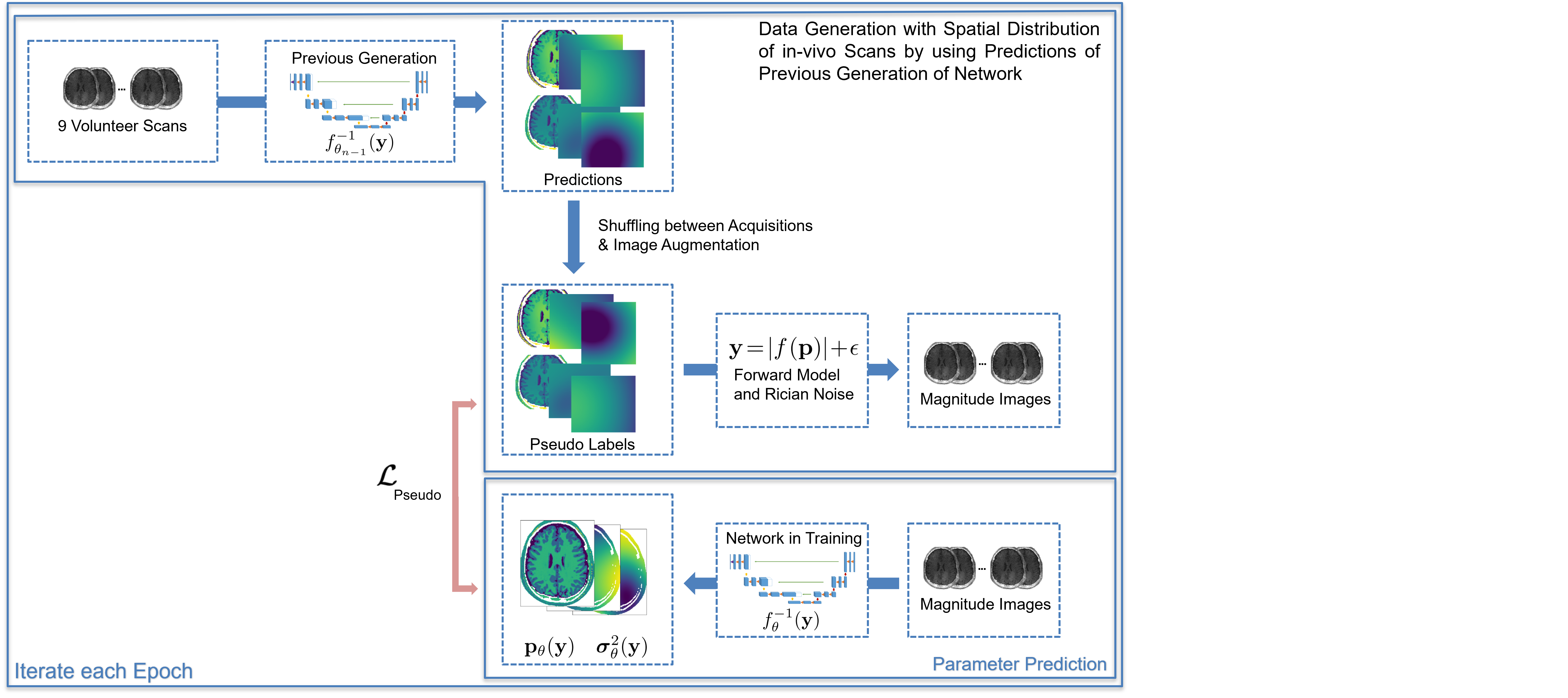
We combined this with pseudo-label training¹⁴ to increase the training data and decrease the correlation bias between the predictions of different parameters (figure 3). In each epoch, we used a combination of the network trained in the previous epoch and the known forward model as a teacher for the network. By separately augmenting and shuffling the estimates of the parameter maps for different in-vivo scans, we created in each epoch a new dataset with labels closer to the true spatial distribution of in-vivo samples compared to our synthetic dataset, while decreasing the correlation between the different parameter estimates compared to the in-vivo data. These labels allowed training on the GNLL-Loss $$$L_\textrm{Pseudo}$$$.

The fine-tuning was performed with batches of 4 synthetic, 12 pseudo-label, and 8 masked in-vivo scans while optimizing on $$$L= L_\textrm{GNLL}+ \lambda_1 L_\textrm{Pseudo} + \lambda_2 L_\textrm{2Self}$$$, with $$$\lambda_1=3$$$ and $$$\lambda_2=2$$$.

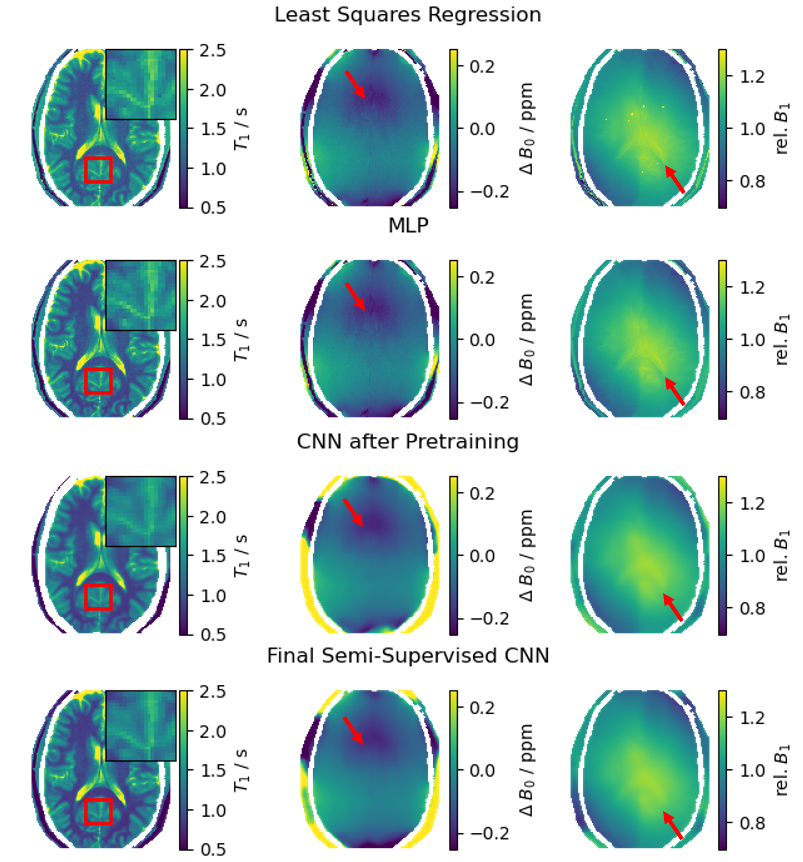
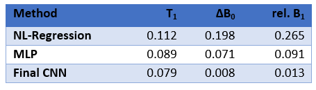
We compare our approach to a non-linear regression as well as a pixelwise neural network³ (MLP)qualitatively on the held-back volunteer scan and quantitatively on a synthetic validation set.

Results

The qualitative results for a randomly selected volunteer chosen for validation are shown in figure 4. The regularization implicitly defined by the selection of generating functions for the synthetic training data results in less (unphysical) cross-talk between the predictions of the different parameters, e.g. the effect of the CSF on the predicted field maps is reduced. The CNN allows for spatial regularisation suppressing noise in the final maps, but can also lead to blurring. With the proposed fine-tuning approach this blurring is strongly reduced while ensuring robust parameter estimation. Using a validation set of purely synthetic data, we calculated the nRMSE of the final fine-tuned model as 0.08 for T₁, 0.008 for the B₀- and 0.013 for the B₁-maps (table 1).

Discussion and Conclusion

We demonstrated the superiority of a spatially regularized deep learning prediction of T₁, B₀, and B₁ from a WASABITI scan compared to pixelwise methods while allowing fast reconstruction. Our semi-supervised approach allowed to make use of the a-priori domain knowledge about typical spatial distributions of the parameter maps, while allowing the adaptation to in-vivo spatial distributions. Our method can easily be extended to under-sampled data and, in principle, be applied to any inverse problem with a known forward model. Further investigation of the suggested fine-tuning routine for adaptation to different distributions and slight imperfections of the forward model will be performed in the future.
Network weights and all code will be made available as open-source.

Acknowledgements

This work was funded within the “Metrology for Artificial Intelligence in Medicine (M4AIM)” project by the German Ministry for Economy and Climate Action as part of the QI-Digital Initiative and by the Heidenhain Foundation in the framework of the Junior Research Group “Machine Learning and Uncertainty”.

References

1. Schuenke, P., Windschuh, J., Roeloffs, V., Ladd, M.E., Bachert, P. and Zaiss, M. Simultaneous mapping of water shift and B1 (WASABI)—application to field‐inhomogeneity correction of CEST MRI data. MRM 77(2), pp.571-580, 2017

2. Deichmann, R. and Haase, A. Quantification of T1 values by SNAPSHOT-FLASH NMR imaging. Journal of Magnetic Resonance, 96(3), pp.608-612, 1992

3. Schuenke, P., Heinecke, K., Narvaez, G., Zaiss, M. and Kolbitsch, C. Simultaneous Mapping of B0, B1 and T1 Using a CEST-like Pulse Sequence and Neural Network Analysis. Joint Annual Meeting ISMRM-ESMRMB & ISMRT. Abstract 2714, 2022

4. Hunger,L., German, A., Glang, F., Khakzar,K., Dang,N., Mennecke, A., Maier, A., Laun, F., and Zaiss, M. DeepCEST: 7T Chemical exchange saturation transfer MRI contrast inferred from 3T data via deep learning with uncertainty quantification. 28th ISMRM & SMRT Annual Meeting & Exhibition, Abstract 1451, 2019

5. Liu, F., Feng, L., and Kijowski, R. MANTIS: Model-Augmented Neural neTwork with Incoherent k-space Sampling for efficient MR parameter mapping. MRM, 82(1), 174–188, 2019

6. Qiu, S., Christodoulou, A., Xie,Y., and Li, D. Hybrid supervised and self-supervised deep learning for quantitative mapping from weighted images using low-resolution labels. 31st Joint Annual Meeting ISMRM-ESMRMB & ISMRT, Abstract 2609, 2022

7. Jeelani, H., Yang, Y., Zhou, R., Kramer, C.M., Salerno, M. and Weller, D.S. A myocardial T1-mapping framework with recurrent and U-Net convolutional neural networks. IEEE 17th International Symposium on Biomedical Imaging (ISBI), 2020

8. Ronneberger, O., Fischer, P. and Brox, T. U-net: Convolutional networks for biomedical image segmentation. In International Conference on Medical image computing and computer-assisted intervention (pp. 234-241), 2015

9. Aubert-Broche, B., Griffin, M., Pike, G.B., Evans, A.C. and Collins, D.L. Twenty new digital brain phantoms for creation of validation image data bases. IEEE transactions on medical imaging, 25(11), pp.1410-1416, 2006

10. Mulkern, R.V. and Williams, M.L. The general solution to the Bloch equation with constant rf and relaxation terms: application to saturation and slice selection. Medical physics, 20(1), pp.5-13, 1993

11. Ravi K, Geethanath S, Vaughan J. PyPulseq: A Python Package for MRI Pulse Sequence Design. J. Open Source Softw.;4:1725, 2019

12. Batson, J. and Royer, L. Noise2self: Blind denoising by self-supervision. In International Conference on Machine Learning (pp. 524-533). PMLR, 2019

13. Yaman, B., Hosseini, S.A.H., Moeller, S., Ellermann, J., Uğurbil, K. and Akçakaya, M. Self‐supervised learning of physics‐guided reconstruction neural networks without fully sampled reference data. MRM 84(6), pp.3172-3191, 2020

14. Chen, W., Lin, L., Yang, S., Xie, D., Pu, S., Zhuang, Y. and Ren, W. Self-supervised noisy label learning for source-free unsupervised domain adaptation. arXiv:2102.11614, 2021

Figures

Figure 1: We generated synthetic labels based on the Brainweb dataset of healthy segmented brains and random B₀- and B₁-field inhomogeneities. We used these labels combined with the analytical expression $$$f$$$ of the forward model and degradation by Rician noise to generate input data and train a U-Net. To estimate the aleatoric uncertainty of our predictions, we model the likelihood by a Gaussian distribution with a heteroscedastic variance, which is also predicted by the network.

Figure 2: We applied a Noise2Self-inspired approach for fine-tuning on in-vivo data by splitting the acquired data in each voxel into input data and labels. The network learns to predict T₁, B₀, and B₁ from the input labels such that applying the forward model results in the best fit for the unseen label data points, thereby avoiding fitting to the noise and instead learning the spatial correlation of the parameters.

Figure 3: To increase the available real data from volunteer scans into our training, we used a teacher-student approach with separately augmented and mixed pseudo-labels generated by a previous generation of our model. As the true field inhomogeneities are mostly uncorrelated to the anatomical relaxation maps, the independent augmentations avoid learning non-realistic correlations.

Figure 4: Comparison of non-linear least square regression, a pixelwise network³ (MLP), the U-Net trained on synthetic data only, and the fine-tuned network (from top to bottom) on one volunteer not used during training. The implicit regularization learned by the U-Net results in less influence of the CSF on the predicted field maps and reduced noise in the T₁ predictions. Fine-tuning (qualitatively) reduces the visible blur in the T₁ maps.

Table 1: Comparison of nRMSE on a synthetic WASABITI validation dataset

Proc. Intl. Soc. Mag. Reson. Med. 31 (2023)

1166

DOI: https://doi.org/10.58530/2023/1166