1144
Direct estimation of pharmacokinetic parameters of DCE-MRI from raw k-space data with model-based reconstruction1Department of Radiology and Nuclear Medicine, Amsterdam University Medical Center, Amsterdam, Netherlands, 2Department of Biomedical Engineering and Physics, Amsterdam University Medical Center, Amsterdam, Netherlands, 3Division of Radiotherapy and Imaging, The Institute of Cancer Research, London, United Kingdom, 4Institute of Medical Engineering, Technical University Graz, Graz, Austria
Synopsis
Keywords: Contrast Agent, Quantitative Imaging, Model-based reconstruction
Dynamic contrast enhanced (DCE) MRI is a minimally invasive technique that is able to quantitatively investigate the tumor vasculature microenvironment. Such information shows great potential for treatment stratification and response monitoring. However, DCE typically suffers from low spatial resolution, Rician noise bias, and errors due to complex perfusion modeling. Model-based reconstruction, in which DCE parameters are estimated directly from k-space, may overcome these shortcomings. In this study, we implemented model-based reconstruction for DCE-MRI data, validated it in simulations, and showed its performance in-vivo. With model-based reconstruction the estimated parameter maps exhibited less noise and preserved more anatomical details.Introduction
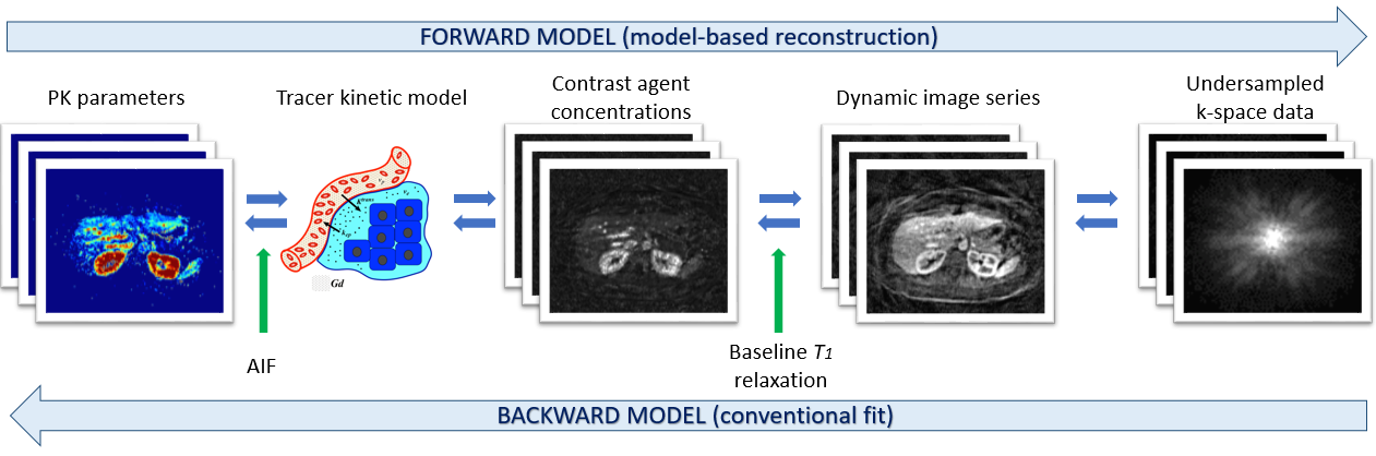
Perfusion and vascularization, as studied by dynamic-contrast enhanced (DCE) MRI, show great potential, e.g. for treatment stratification and response monitoring in cancer patients(1-3). However, the quantification of DCE-MRI data faces several challenges hampering its introduction to clinical practice. First, the need to fill sufficient k-space to produce dynamic images generates a trade-off between temporal resolution, needed to capture the complex contrast dynamics, and spatial resolution, desired for accurately depicting the tumor. Second, the Rician-distribution of noise in the image domain introduces a noise-dependent bias to quantified parameters. Third, due to complex modeling, quantitative perfusion estimations show high variance. These shortcomings result in large day-to-day variations and sequence-dependent biases in estimations, preventing routine clinical use of DCE.Model-based reconstruction (MBR) has the potential to overcome these challenges. MBR includes a biophysical model mapping quantitative parameters back to the signal in the k-space (Figure 1), rather than just to the conventional image space. The inverse problem associated with the model is solved with an iterative approach that compares measured k-space data to results of the forward modeling of the estimated parameters. MBR removes the noise-dependent bias, as noise is Gaussian in k-space. Furthermore, MBR no longer has the implicit trade-off between temporal and spatial resolution as the need for intermediate images is removed.
Therefore, we implemented the extended Tofts DCE model in the PyQMRI MBR framework(4), validated its performance in a digital phantom (XCAT(5)), mimicking DCE-MRI in the abdominal region, showed its feasibility in-vivo, and compared it to the conventional nonlinear least squares fitting (LSQ).
Methods
For the modeling of pharmacokinetic (PK) parameters, the Extended Tofts model was used(6). Estimated PK parameters included fractional plasma volume (vp), the fractional volume of extracellular extravascular space (EES) (ve), and the mass reflux rate from EES back into plasma (kep). A population-based arterial input function was used and treated in analytical representation allowing for analytical integration(7).We implemented the Extended Tofts model for DCE in the PyQMRI framework for MBR(4). PyQMRI applies an iteratively regularized Gauss-Newton approach combined with a primal-dual inner loop for the non-linear fitting. A total generalized variation functional was used as a regularization strategy(8). The forward model was based upon the contribution by Orton et al. to the OSIPI GitHub(9). In MBR the forward model mapped PK parameters directly to the k-space data.
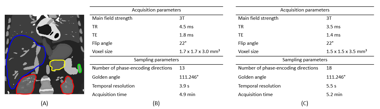
A 2D coronal plane of the extended Cardiac-Torso anatomical (XCAT) phantom was used for validation(5) (Figure 2A). Several organs from the phantom were selected for our simulations: liver, pancreas, spleen, and kidneys. The simulation of DCE-MRI signal was calculated using a forward model based on the PK parameters from the literature for all organs except for the kidneys, which were estimated from healthy volunteers scanned at our center(10) (Figure 4B). For simplicity, the baseline T1 map was considered to be constant over the image and equal to 700ms. A golden angle radial undersampling trajectory was simulated for which the scan and sampling parameters are listed in Figure 2B. The noise in simulations was considered to be caused by undersampling only. Additionally, two 2D axial planes from scans of healthy volunteers were used to show MBR’s feasibility in vivo (Figure 2C).
As a comparison to MBR, a conventional analysis with a NUFFT followed by voxel-wise nonlinear LSQ fit was performed. The mean values and standard deviation of predicted PK parameters were calculated in simulations for both methods.
Results
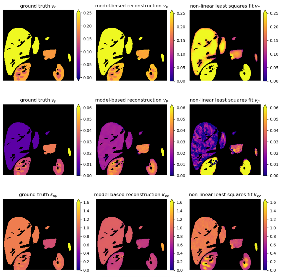
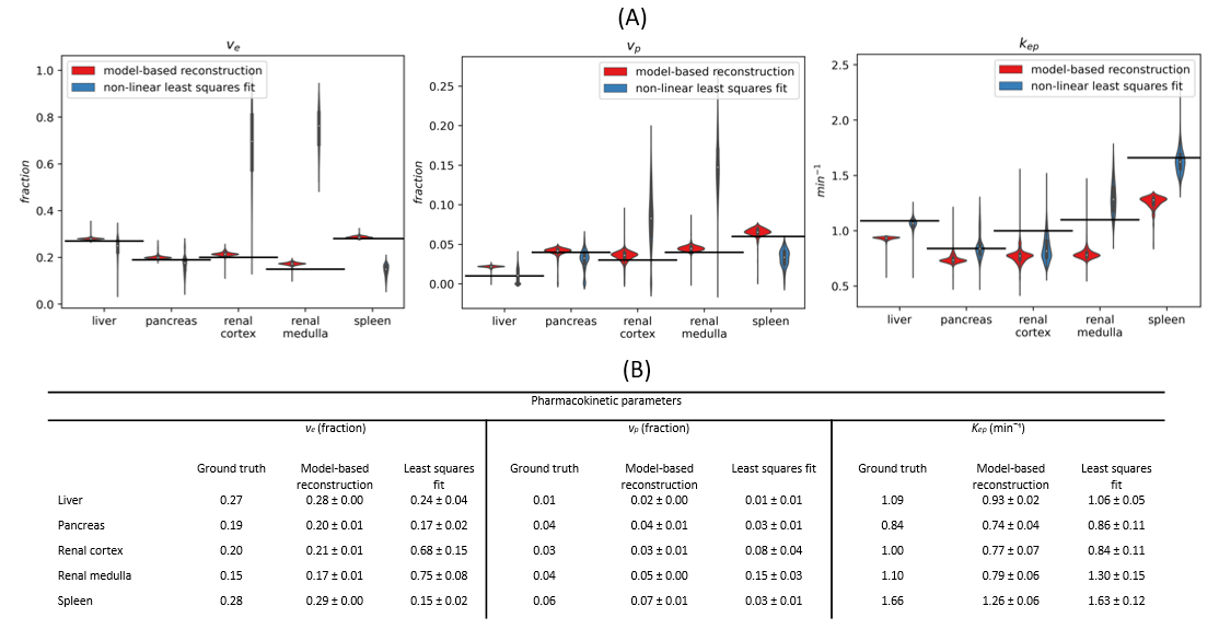
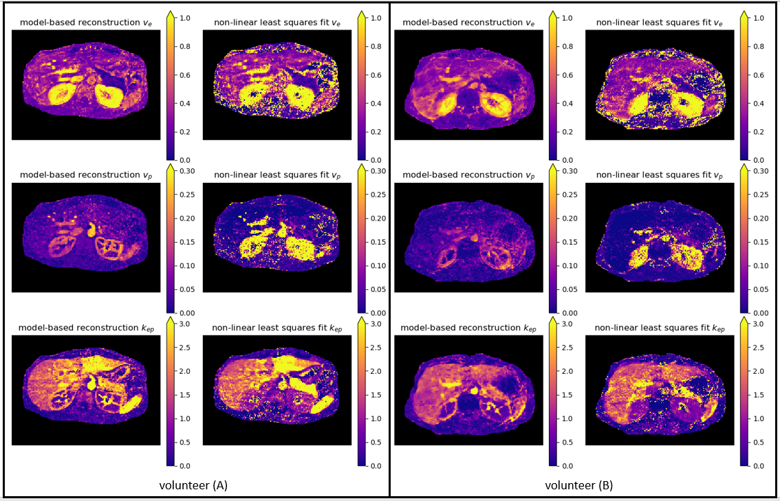
MBR successfully estimated PK parameters and resulted in more homogenous (less noisy) parameters within each organ than the LSQ reference, which was especially visible in vp map in the liver (Figure 3). MBR resulted in less bias and smaller spread in parameter values in 9 out of 15 organ/parameter combinations (Figure 4). The accuracy of estimated PK parameters in small anatomical regions, such as in renal medulla, was higher or equal with MBR.In vivo we have similar observations as in the simulations: quantitative maps were more homogeneous and better depicted smaller anatomical objects when estimated with MBR (Figure 5). Additionally, the border of different organs is more clearly visible on MBR maps which might be important for the delineation of anomaly.
Discussion
In this work, we implemented MBR for DCE-MRI and validated it in a digital phantom and in vivo. We showed that MBR removes the noise-dependent bias due to direct reconstruction from raw k-space and is robust to random errors due to regularization. Furthermore, small anatomical details and borders of organs were better distinguishable with MBR. Given these results, MBR has the potential to achieve better scan-rescan repeatability, which is essential in daily clinical practice.In this study, the regularization weight was tuned based on visual impression. A systematic optimization could further improve the results. Moreover, we used the same T1 relaxation time for all organs. Including T1 in the fitting is desirable since it varies per tissue and could influence PK parameters. Lastly, the conventional LSQ fitting is not a state-of-the-art method, and a comparison with more advanced algorithms is recommended.
In the future, a detailed comparison of MBR and conventional fitting will be investigated in vivo.
Conclusion
MBR for DCE-MRI can be used to substantially improve PK map quality.Acknowledgements
This research has been financed by KWF-UVA 2021.13785 and CCA 2020-7-01.
References
1. Counago F, del Cerro E, Diaz-Gavela AA, Marcos FJ, Recio M, Sanz-Rosa D, et al. Tumor staging using 3.0 T multiparametric MRI in prostate cancer: impact on treatment decisions for radical radiotherapy. Springerplus. 2015;4.
2. Jahani N, Cohen E, Hsieh MK, Weinstein SP, Pantalone L, Hylton N, et al. Prediction of Treatment Response to Neoadjuvant Chemotherapy for Breast Cancer via Early Changes in Tumor Heterogeneity Captured by DCE-MRI Registration. Sci Rep-Uk. 2019;9.
3. Wang CH, Yin FF, Horton J, Chang Z. Review of treatment assessment using DCE-MRI in breast cancer radiation therapy. World J Methodol. 2014;4(2):46-58.
4. Maier O, Spann SM, Bödenler M, Stollberger R. PyQMRI: an accelerated Python based quantitative MRI toolbox. Journal of Open Source Software. 2020;5(56):2727.
5. Wissmann L, Santelli C, Segars WP, Kozerke S. MRXCAT: Realistic numerical phantoms for cardiovascular magnetic resonance. J Cardiovasc Magn R. 2014;16.
6. Tofts PS. Modeling tracer kinetics in dynamic Gd-DTPA MR imaging. Jmri-J Magn Reson Im. 1997;7(1):91-101.
7. Orton MR, d'Arcy JA, Walker-Samuel S, Hawkes DJ, Atkinson D, Collins DJ, et al. Computationally efficient vascular input function models for quantitative kinetic modelling using DCE-MRI. Phys Med Biol. 2008;53(5):1225-39.
8. Bredies K, Kunisch K, Pock T. Total generalized variation. SIAM Journal on Imaging Sciences. 2010;3(3):492-526.
9. Orton MR, Gurney-Champion OJ. OSIPI. 2021 [Available from: https://github.com/OSIPI/DCE-DSC-MRI_CodeCollection/tree/develop/src/original/OG_MO_AUMC_ICR_RMH_NL_UK].
10. Holland MD, Morales A, Simmons S, Smith B, Misko SR, Jiang XY, et al. Disposable point-of-care portable perfusion phantom for quantitative DCE-MRI. Medical Physics. 2022;49(1):271-81.
Figures