1103
In vivo Multi-Parameter Mapping of the Habenula using MRI1Wellcome Centre for Human Neuroimaging, University College London, London, United Kingdom, 2Harvard Medical School, Boston, MA, United States, 3Institute of Cognitive Neuroscience, University College London, London, United Kingdom
Synopsis
Keywords: Quantitative Imaging, Tissue Characterization, Multi-Parameter Mapping
The habenula has attracted much interest in neuroscience studies because it plays an important role in the reward circuitry of the brain and is implicated in psychiatric conditions. However, imaging the habenula remains challenging due to its sub-cortical location and small size, with few reports analysing its microstructural composition in vivo. To address this gap in the literature, we performed a multi-parametric characterisation of the microstructure of the habenula by quantifying relaxation rates (R1, R2*), water content (PD) and a marker of macromolecular content (MTsat), most notably myelin, in a cohort of 20 healthy participants.Introduction
The habenula is a small, epithalamic brain structure1 that plays an important role in the reward circuitry of the brain and is implicated in psychiatric conditions, such as depression1–3. The importance of the habenula for human cognition and mental health make it a key structure of interest for neuroimaging studies. However, relatively few studies have been conducted in humans because habenula visualization in vivo is challenging, due to its subcortical location and small size. Studies to date have focused on characterizing the morphology4,5, connectivity6–8 or functional role3,9–11 of the habenula, but few reports have characterized its physical properties.Microstructural characterization of the habenula to date has focused on quantitative susceptibility mapping (QSM)12,13. In this work, we complement this with measures of the longitudinal and effective transverse relaxation rates (R1 and R2* respectively), proton density (PD) and magnetisation transfer saturation (MTsat) using a high-resolution (0.8mm isotropic) quantitative multi-parametric mapping (MPM) protocol at 3T, in a cohort of 20 healthy participants.
Methods
In vivo AcquisitionsData were acquired on a Siemens 3T Prisma using a 64-channel head and neck receiver coil using an MPM protocol14. It comprised three RF- and gradient-spoiled multi-echo 3D FLASH scans acquired with T1 (αT1w = 21°), PD (αPDw = 6°) or MT (αMTw = 6°) weighting. A Gaussian RF pulse at 2kHz off-resonance with flip angle of 220˚ was used to achieve MT-weighting. A transmit field map was acquired prior to the acquisition of the 3D FLASH scans to account for inhomogeneity15.
Data Analysis
R1, R2*, PD and MTsat maps were generated for each participant using the hMRI toolbox16. The habenula region of interest (ROI) was delineated on the R1 maps following the geometric approach described by Lawson et al.17. For each participant the mean and standard deviation of R1, R2*, PD and MTsat were computed within the habenulae ROI (including both the left and right habenulae). The average volume of the left and right habenulae was also computed for each participant. Participant-specific grey matter (GM) masks including GM surrounding both the left and right habenula were defined and CNR between the habenula and the GM ROI was calculated for each map. Spatial normalization of the R1, R2*, PD, MTsat, GM probability maps and binarised habenulae ROI was performed using the Dartel toolbox in SPM18. The CNR between the habenula and surrounding GM defined in normalized space was calculated on the cohort-averaged R1, R2*, PD and MTsat maps varying the probability threshold (across the cohort) defining the habenula.
Results
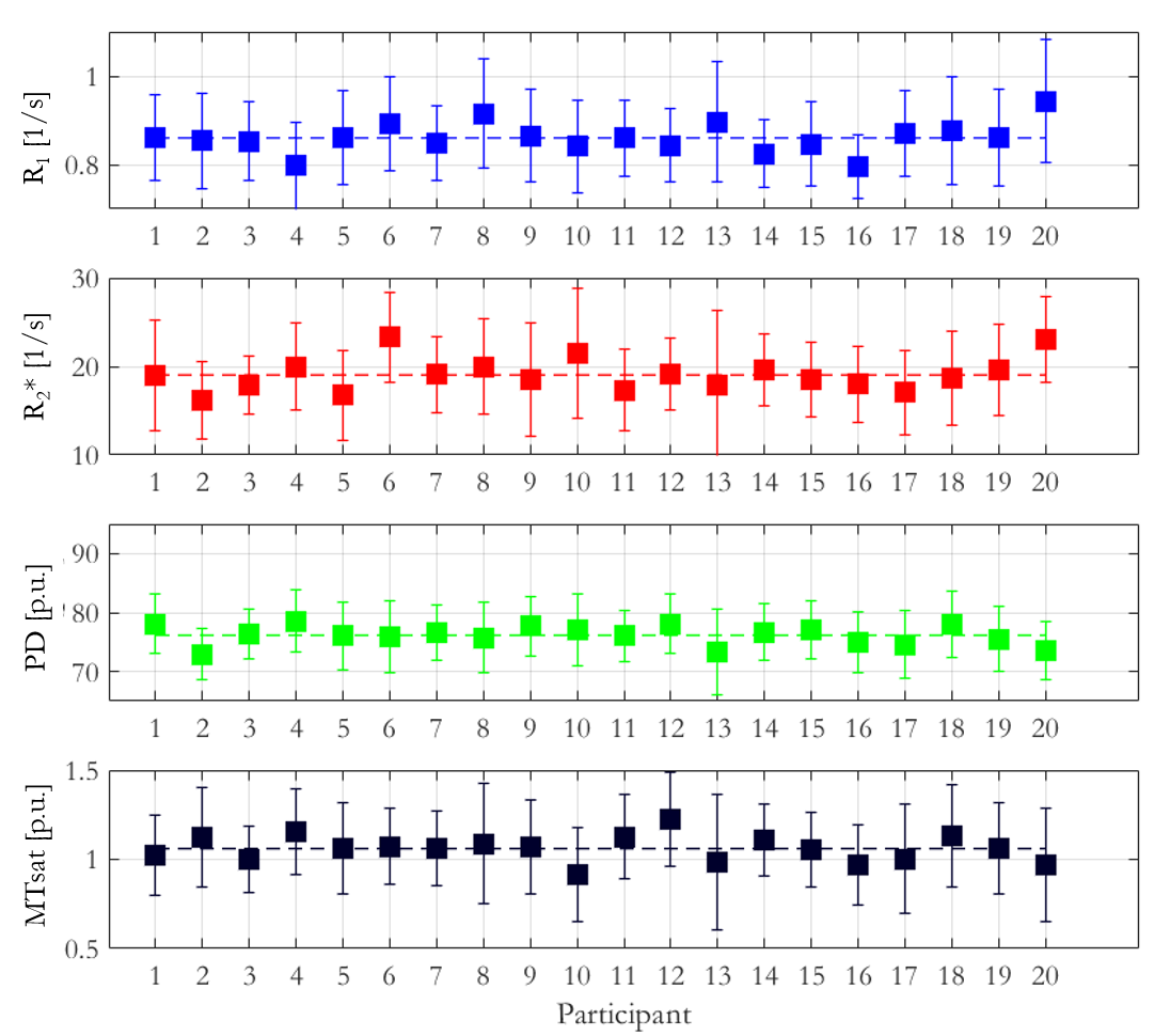
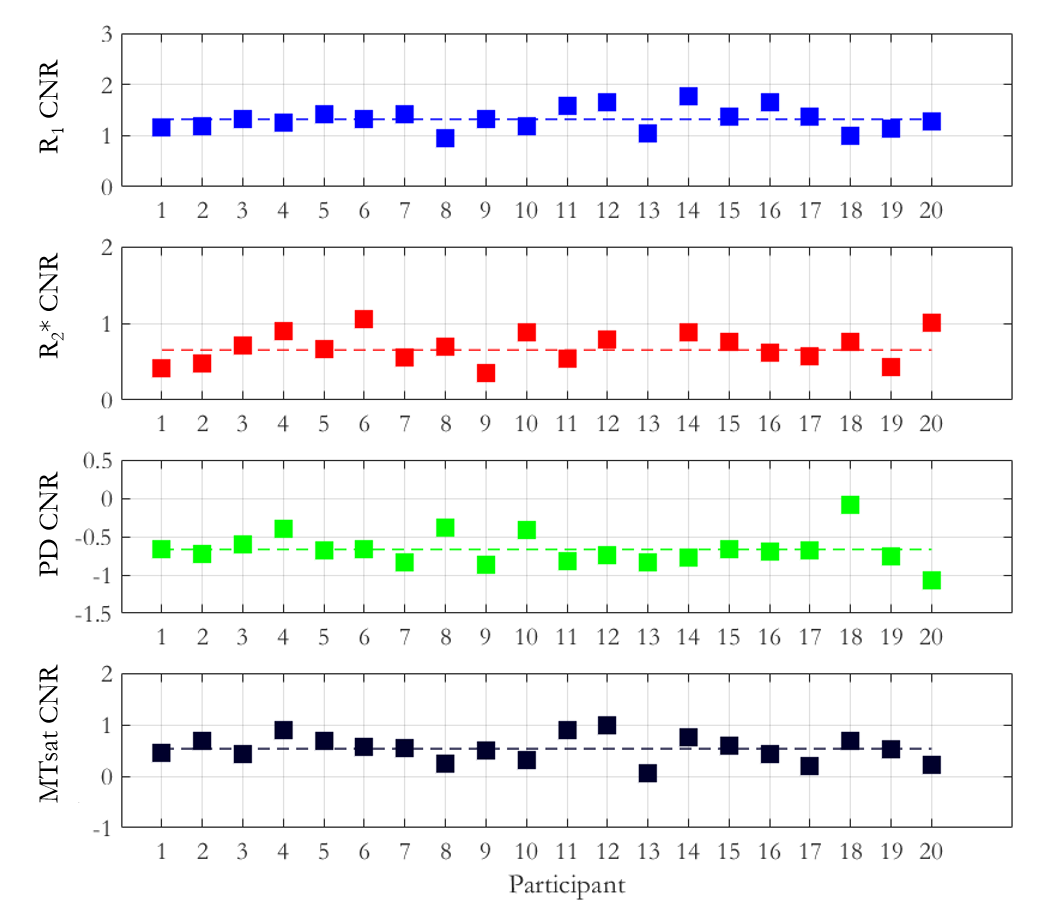
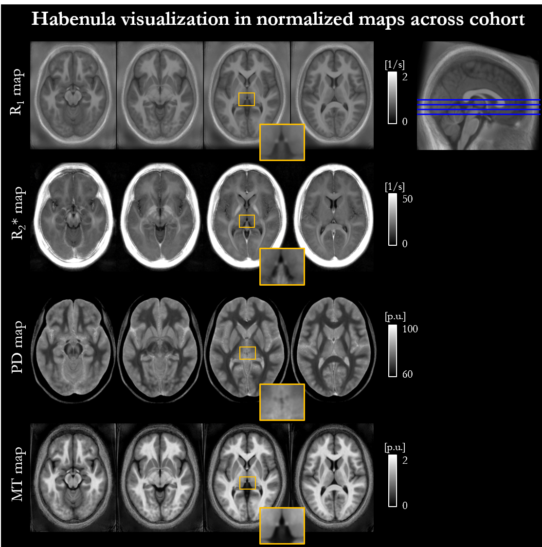
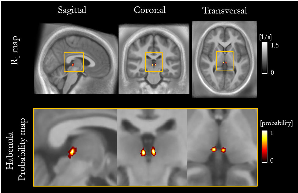
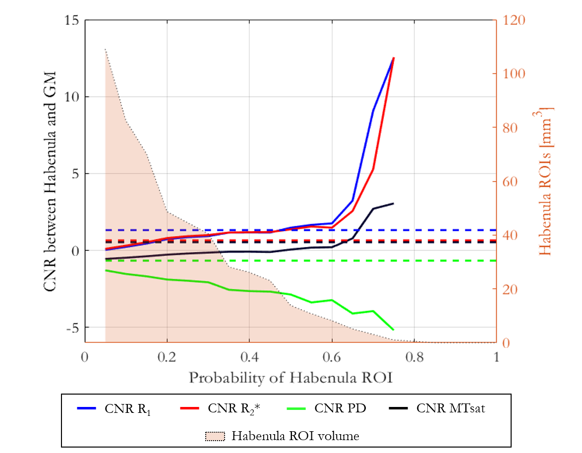
The mean ± standard deviation (std) of the parameters, across participants, within this habenula ROI was R1 = 0.86±0.03 1/s, R2* = 19.04±1.88 1/s, PD = 76.14±1.62 % and MTsat = 1.06±0.07 % (Figure 1). The averaged left and right habenula volumes of each participant were computed. The mean ± std, across participants, of this averaged volume was 18.91±2.13 mm3 with similar left (19.32±2.78 mm3) and right (18.48±2.29 mm3) habenula volumes. The CNR measured between the habenula and the surrounding GM per participant are shown in Figure 2. The R1 maps had the highest CNR with a mean ± std across participants of 1.32±0.22. The R2* and MTsat maps also had positive CNR at 0.65±0.25 and 0.53±0.25 respectively. On the PD maps, the habenula was hypointense relative to the surrounding GM leading to a negative CNR of -0.67±0.21.The cohort-average maps are shown in Figure 3 along with a zoomed view focusing on the habenula. Figure 4 indicates the probability, for this cohort, that a voxel lies within the habenula, superimposed on the cohort-average R1 map. The maximum probability was 0.80 which amounts to only one voxel being consistently defined as being within the habenula for 16 of the 20 participants. CNR was also computed on the cohort-average maps in normalized space (Figure 5). The R1 maps had highest CNR and as the definition of the habenula became more conservative (higher probability of being within the habenula) the CNR increased.
Discussion
In this work, we performed a multi-parametric characterisation of the microstructure of the habenula by quantifying relaxation rates (R1, R2*), water content (PD) and a marker of macromolecular content (MTsat), most notably myelin, in a cohort of 20 healthy participants. The measurements were consistent across the cohort and could therefore be used to guide future studies optimising the in vivo visualisation of the habenula. The habenula was most clearly visualised on the R1 map and its boundaries were consistent across the different parameter maps. CNR analyses confirmed that the contrast between the habenula and the surrounding GM was consistently highest on the R1 maps for each participant. The CNR analysis on the normalized maps reflected what was observed on a per-participant basis. Despite the high CNR observed in normalised space, the overlap of the habenula across the cohort was poor as evidenced by the probability map. Further information related to this work can be found in the following preprint: https://www.researchsquare.com/article/rs-2159322/v1.Acknowledgements
This research was funded in whole, or in part, by the Wellcome Trust [203147/Z/16/Z].References
1. Matsumoto M, Hikosaka O. Lateral habenula as a source of negative reward signals in dopamine neurons. Nature. 2007;447(7148):1111-1115. doi:10.1038/nature05860
2. Tian J, Uchida N. Habenula lesions reveal that multiple mechanisms underlie dopamine prediction errors. Neuron. 2015;87(6):1304-1316. doi:10.1016/j.neuron.2015.08.028.Habenula
3. Lawson RP, Nord CL, Seymour B, et al. Disrupted habenula function in major depressive disorder. Mol Psychiatry. 2017;22(2):202-208. doi:10.1038/mp.2016.81
4. Savitz JB, Nugent AC, Bogers W, et al. Habenula volume in bipolar disorder and major depressive disorder: A high-resolution magnetic resonance imaging study. Biol Psychiatry. 2011;69(4):336-343. doi:10.1016/j.biopsych.2010.09.027
5. Bianco IH, Wilson SW, Adrio F, et al. The habenular nuclei: a conserved asymmetric relay station in the vertebrate brain. Philos Trans R Soc Lond B Biol Sci. 2009;364(1519):1005-1020. doi:10.1098/rstb.2008.0213
6. Ely BA, Xu J, Goodman WK, Lapidus KA, Gabbay V, Stern ER. Resting-state functional connectivity of the human habenula in healthy individuals: Associations with subclinical major depressive disorder. Hum Brain Mapp. 2016;37(7):2369-2384. doi:10.1002/hbm.23179
7. Hikosaka O. The habenula: From stress evasion to value-based decision-making. Nat Rev Neurosci. Published online 2010. doi:10.1038/nrn2866
8. Sutherland RJ. The dorsal diencephalic conduction system: a review of the anatomy and functions of the habenular complex. Neurosci Biobehav Rev. 1982;6(1):1-13.
9. Liu WH, Valton V, Wang LZ, Zhu YH, Roiser JP. Association between habenula dysfunction and motivational symptoms in unmedicated major depressive disorder. Soc Cogn Affect Neurosci. 2017;12(9):1520-1533. doi:10.1093/scan/nsx074
10. Furman DJ, Gotlib IH. Habenula responses to potential and actual loss in major depressive disorder: Preliminary evidence for lateralized dysfunction. Soc Cogn Affect Neurosci. 2016;11(5):843-851. doi:10.1093/scan/nsw019
11. Roiser JP, Levy J, Fromm SJ, et al. The Effects of Tryptophan Depletion on Neural Responses to Emotional Words in Remitted Depression. Biol Psychiatry. 2009;66(5):441-450. doi:10.1016/j.biopsych.2009.05.002
12. Lee S-K, Yoo S, Bidesi AS. Reproducibility of human habenula characterization with high-resolution quantitative susceptibility mapping at 3T. In: ISMRM. ; 2017.
13. Schenck J, Graziani D, Tan ET, et al. High Conspicuity Imaging and Initial Quantification of the Habenula on 3T QSM Images of Normal Human Brain. In: ISMRM. Vol 72. ; 2015:2568.
14. Callaghan MF, Josephs O, Herbst M, Zaitsev M, Todd N, Weiskopf N. An evaluation of prospective motion correction (PMC) for high resolution quantitative MRI. Front Neurosci. 2015;9(MAR):1-9. doi:10.3389/fnins.2015.00097
15. Lutti A, Stadler J, Josephs O, et al. Robust and fast whole brain mapping of the RF transmit field B1 at 7T. PLoS One. 2012;7(3):1-7. doi:10.1371/journal.pone.0032379
16. Tabelow K, Balteau E, Ashburner J, et al. hMRI – A toolbox for quantitative MRI in neuroscience and clinical research. Neuroimage. 2019;194(December 2018):191-210. doi:10.1016/j.neuroimage.2019.01.029
17. Lawson RP, Drevets WC, Roiser JP. Defining the habenula in human neuroimaging studies. Neuroimage. 2013;64(1):722-727. doi:10.1016/j.neuroimage.2012.08.076
18. Ashburner J. A fast diffeomorphic image registration algorithm. Neuroimage. 2007;38(1):95-113. doi:10.1016/j.neuroimage.2007.07.007
Figures