1090
Diving into Extended Phase Graph-based Deep Learning for accurate T2 mapping with PENGUIN1Institute for Systems and Robotics - Lisboa and Department of Bioengineering, Instituto Superior Técnico – Universidade de Lisboa, Lisbon, Portugal, Lisbon, Portugal, 2School of Biomedical Engineering and Imaging Sciences, King’s College London, United Kingdom, London, United Kingdom, 3Center of Marine Sciences - CCMAR, Faro, Portugal, Faro, Portugal, 4Centre for the Developing Brain, School of Biomedical Engineering and Imaging Sciences, King's College, London, UK, London, United Kingdom
Synopsis
Keywords: Quantitative Imaging, Relaxometry
Model-based deep learning approaches have shown promising results to accelerate T2 relaxometry, but most adopt a pure exponential curve to model the signal, which does not account for indirect and stimulated echoes. A PhasE graph sigNal and Gradients QUantitative Inference MachiNe (PENGUIN) is proposed, which implements a dictionary of pre-calculated echo-modulation curves following the Extended Phase Graph (EPG) formulation and respective gradients as the inputs of a Recurrent Inference Machine to perform accurate T2 mapping from the reconstructed images. PENGUIN is 25-fold faster than a pattern recognition approach with a T2 dictionary step of 2 ms.
Introduction
Quantitative Magnetic Resonance Imaging often suffers from time-consuming parameter fitting operations, preventing its use in routine clinical evaluation. A new class of deep learning frameworks, called model-based deep learning nets, incorporate the MR signal model into the learning process to estimate parametric maps of the tissues, alleviating the need for a large number of training datasets and further pushing acceleration rates [1]. However, most of the previously proposed methods have employed a pure exponential curve to model the MR signal [2,3], which does not account for stimulated or indirect echoes, or inhomogeneity of the B1 field. Here, the PhasE graph sigNals and Gradients qUantitative Inference machiNe (PENGUIN) method is proposed, which adapts the Recurrent Inference Machine (RIM) implemented by Sabidussi et al. [3] (model-based method), to perform T2 mapping of grey and white matter regions with a more accurate signal model based on the Extended Phase Graphs (EPG) concept [4], while also attempting to estimate the effective B1 field to improve the T2 map estimate. In addition to the new signal model, a key difference between PENGUIN and RIM is that an efficient dictionary implementation is used to obtain the forward signal model and corresponding gradients to speed up the estimation.Methods
All methods were implemented with a signal model based on the EPG concept, following a multi echo spin-echo (ME-SE) acquisition sequence, with 32 echoes, TE=10:10:320 ms and flip angle (FA) = [180°, 160°, … 160°], by modifying the code by Sabidussi et al [3]. A dictionary of echo-modulation curves (EMC) with the EPG formulation and corresponding gradients was built for T2 = 0:1:2000 ms, B1 = 0.6:0.01:1.4, and T1 = 1000 ms.Pattern-recognition approach: A state-of-the-art pattern-recognition approach was implemented by looping through each pixel of the reconstructed images and attributing to it the T2 value of the dictionary whose EMC maximized its inner product with the measured signal of that pixel.
PENGUIN: PENGUIN was implemented according to the configuration in Figure 1. At each optimization step, the network performs $$$J$$$=6 inference steps to obtain 6 estimates of the parametric maps $$$\hat{\textbf{p}}$$$=[PD, T2, B1], where PD is a tissue-dependent normalization constant, including the proton density. The loss function was given by: $$\Lambda^{total} = \frac{1}{J} \sum_{j=1}^J \left(\sum (\textbf{p}-\hat{\textbf{p}_j})^2\right).$$
PENGUIN finds the maximum a posteriori estimate of the signal $$$\textbf{m}$$$, from which the negative log-likelihood function $$$\mathcal{L}(\textbf{m} | \textbf{p})$$$ can be defined, while implicitly learning prior information. At each inference step, the network receives the parametric maps $$$\hat{\textbf{p}}_j$$$, the gradient of the negative log-likelihood function $$$\nabla_{\hat{\textbf{p}}_j} \mathcal{L}(\textbf{m} | \hat{\textbf{p}}_j)$$$ and two vectors of memory states $$$\textbf{h}^1_j$$$ and $$$\textbf{h}^2_j$$$ as input, and outputs the incremental update to the maps, $$$\Delta \hat{ \textbf{p}}_j$$$, and the updated vectors of memory states $$$\textbf{h}^1_{j+1}$$$ and $$$\textbf{h}^2_{j+1}$$$. During evaluation, PENGUIN uses the dictionary to speed up the calculation of $$$\hat{\textbf{m}}_j$$$ and $$$\nabla_{\hat{\textbf{p}}_j} \mathcal{L}(\textbf{m} | \hat{\textbf{p}}_j)$$$ compared to the reference RIM implementation.
PENGUIN and RIM networks were implemented with PyTorch 1.10.2, trained on a NVIDIA TESLA P100 GPU, and tested on an Intel Core i7 2.8 GHz CPU. All networks were trained using the Adam optimizer, a learning-rate of 0.005, and 72 patches per minibatch, for a total of 120 epochs.
Simulated Data: Networks were fully trained with simulated data from ten BrainWeb’s discrete anatomical images [5]. Each 3D image was randomly split into 7200 2D patches, from which a set of ground truth $$$\textbf{p}$$$ maps and corresponding T2 weighted images $$$\textbf{m}$$$ were simulated with the EPG implementation, following the scheme in Figure 2. Two additional simulated images were created to test the networks, following the same protocol but considering the full slice (Figure 3).
In vivo Data: PENGUIN was tested and compared to the pattern recognition method on in vivo images of a healthy subject previously acquired in a Philips Achieva 3T scanner with the ME-SE sequence detailed above, imaging 6 slices with spatial resolution of 1.6×1.6×4.0 mm3, field-of-view 250×250 mm2, and repetition time of 4 s.
Results
PENGUIN can estimate a 320×320 pixel map in 4.16±0.10 s, 380-fold faster than the RIM implemented with the EPG signal model while achieving the same accuracy (Figure 4), and 465-fold faster than the pattern recognition approach. Even when considering the latter approach with a coarser dictionary built with T2=0:2:300 ms, PENGUIN is 25 times faster. The T2 maps estimated in the simulated images prove PENGUIN is capable of estimating known T2 values, albeit with less accuracy than the pattern recognition approach. The T2 maps estimated with PENGUIN in the in vivo images (Figure 5) have a maximum median difference of 2.8 ms in the brain parenchyma compared to those obtained with the pattern recognition approach, with a larger error in the grey matter region.Conclusions
PENGUIN provides a faster and reliable alternative to estimate T2 maps, by combining the advantages of the RIM (low overfitting and ability to learn the inference process) and the pattern recognition approach (use of pre-calculated dictionaries with the signal evolution and its derivatives).Acknowledgements
This research was supported by: NVIDIA GPU hardware grant; “la Caixa” Foundation and FCT, I.P. under the project code [LCF/PR/HR22/00533]; FCT through projects UIDB/04326/2020, UIDP/04326/2020, LA/P/0101/2020 and UID/EEA/50009/2020.
References
[1] L. Feng et al, NMR in Biomedicine, 2022, 35:e4416.
[2] F. Liu et al, Magnetic Resonance Imaging, 2020, 74:152–160.
[3] E. R. Sabidussi et al, Medical Image Analysis, 2021, 74:102220.
[4] M. Weigel. Journal of Magnetic Resonance Imaging, 2015, 41:266–295.
[5] C.A. Cocosco et al, NeuroImage, 1997, 5:425.
Figures
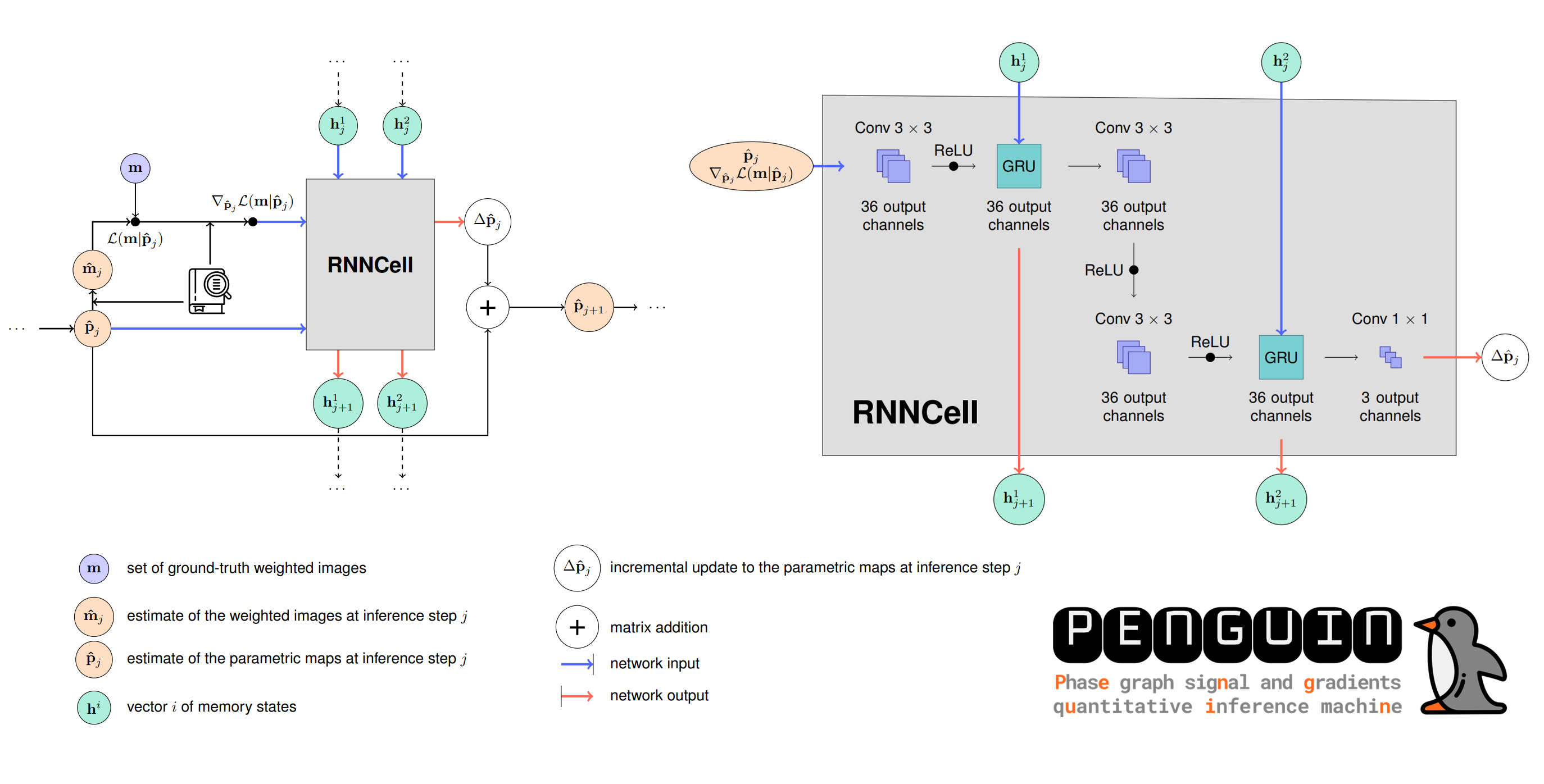
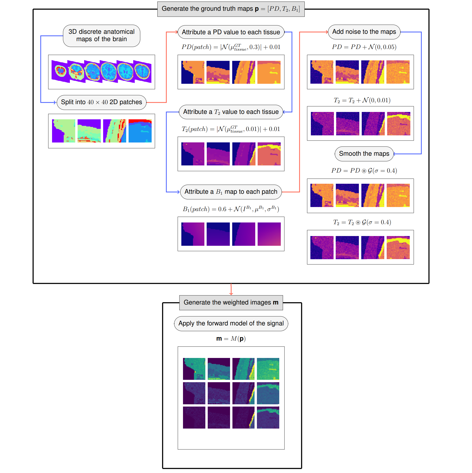
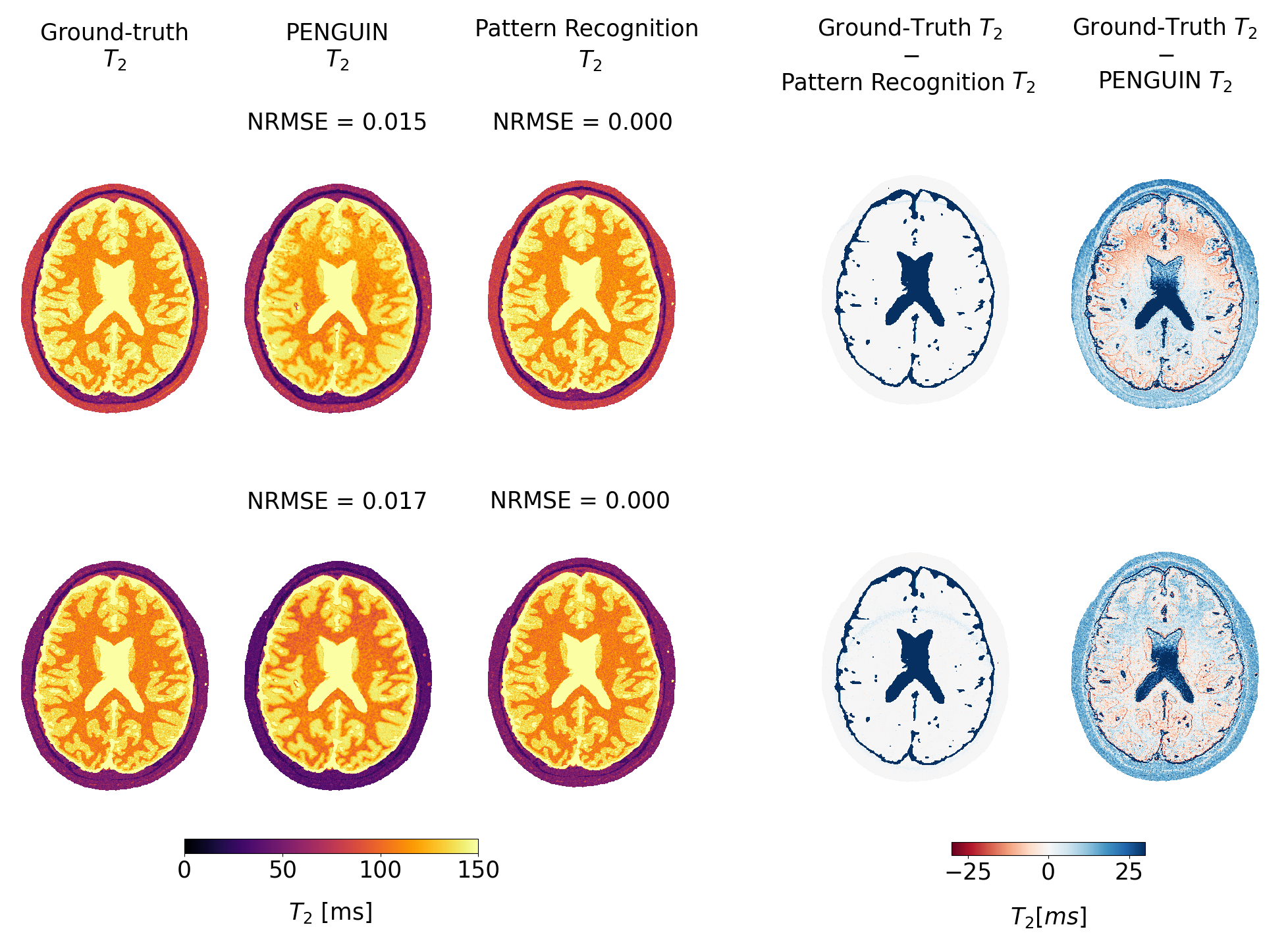
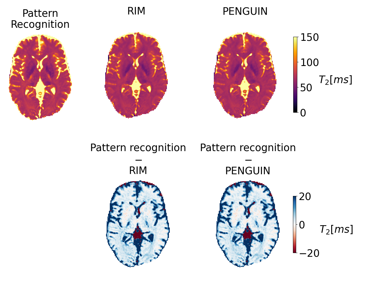
Figure 4: T2 maps estimated with the pattern recognition approach, the RIM implemented with the EPG model, and with PENGUIN (top), and difference maps between the deep learning methods and the pattern recognition method (bottom). PENGUIN and RIM present similar accuracies compared to the standard dictionary approach. However, PENGUIN (4.16±0.10 s) is 380 times faster than RIM (1578±82 s) and 465 times faster than the pattern recognition approach (1931±130 s).
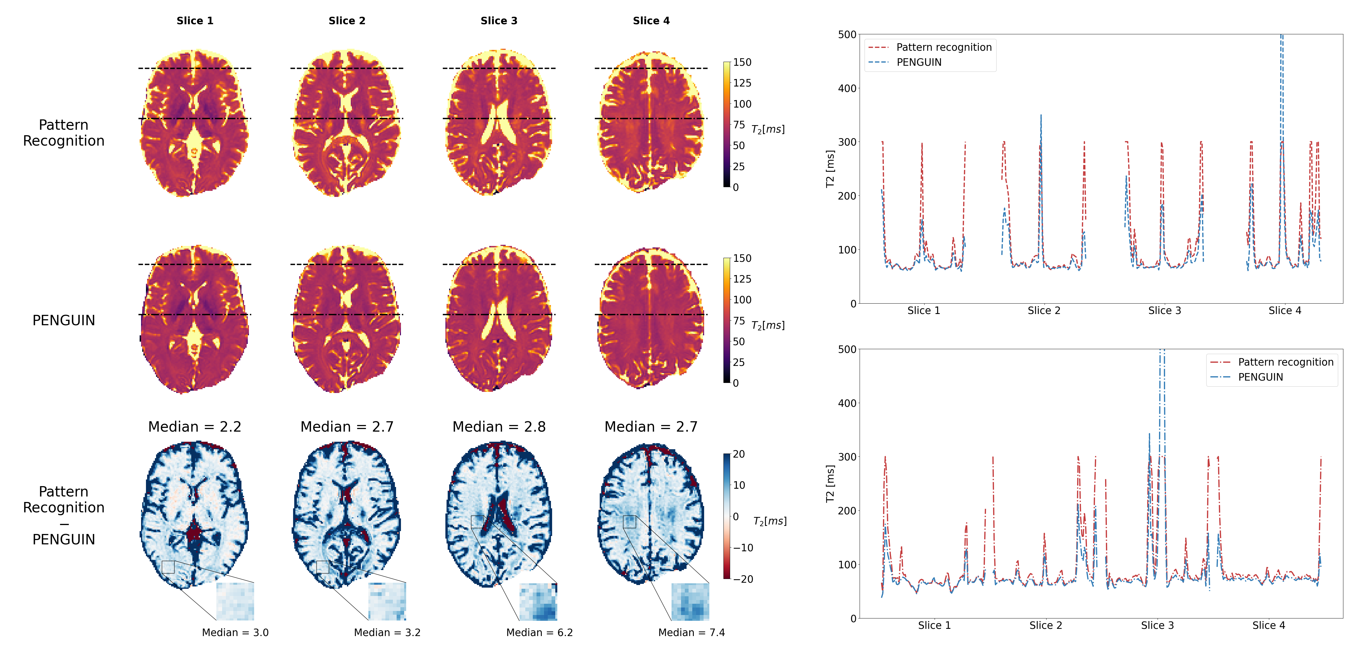
Figure 5: (Left) T2 maps estimated from in vivo weighted images, each column corresponding to a different slice, with the pattern recognition approach with 1 ms T2 dictionary step (top) and with PENGUIN (middle), and difference map between them (bottom). The median error (in ms) was calculated in the brain parenchyma region, excluding the CSF. (Right) Estimated T2 values with both methods alongside two horizontal profiles indicated in the slices.