Synopsis

Keywords: Quantitative Imaging, Quantitative Susceptibility mapping

In this abstract we demonstrate a simple framework that builds up on deep learning infrastructure to perform quantitative susceptibility mapping and correct for susceptibility related effects on R2* maps, taking the advantage of high GPU computational efficiency. Asking the Adam optimizer to point you in the right direction results in a gradient descent method that can perform field mapping, background field removal, QSM and reduce macroscopic intravoxel dephasing artifacts in R2* maps with most operations being performed in under 60 seconds even for 0.8mm isotropic whole brain multi-echo data.

Introduction

Multi-echo Gradient-echo data is frequently used for apparent transverse relaxation rate ($$$R_2^*$$$) and quantitative susceptibility mapping (QSM). Typically, these problems are tackled separately: magnitude and phase data are used to compute $$$R_2^*$$$ and susceptibility ($$$\chi$$$) maps respectively. Yet these two processes are highly intertwined.

Spatial phase variation across voxels causes additional intravoxel dephasing, resulting in an overestimation of $$$ R_2^*$$$. This effect can be alleviated in 3D GRE acquisitions if the voxel spread function is considered, (1) albeit the process is extremely time consuming due to the multiple local deconvolution steps. Meanwhile, obtaining QSM by directly fitting the complex multi-echo data, although not straightforward (2) has advantages over conventional frequency mapping fitting: it correctly accounts for SNR and data fitting errors in the data consistency (particularly important at low SNR).

The Adam optimizer (3) is a stochastic gradient descent optimization algorithm used in deep learning to perform network updates. Its main attributes include: high efficiency, small memory demand, suitability to handle large non-convex problems. It is thus an ideal candidate for relaxometry on full 4D dataset without requiring linearizations that distort the noise appearance, causing biases (4). In this work we highlight 3 applications: Background Field Computation, QSM and signal dropout $$$R_2^*$$$ correction.

Methods

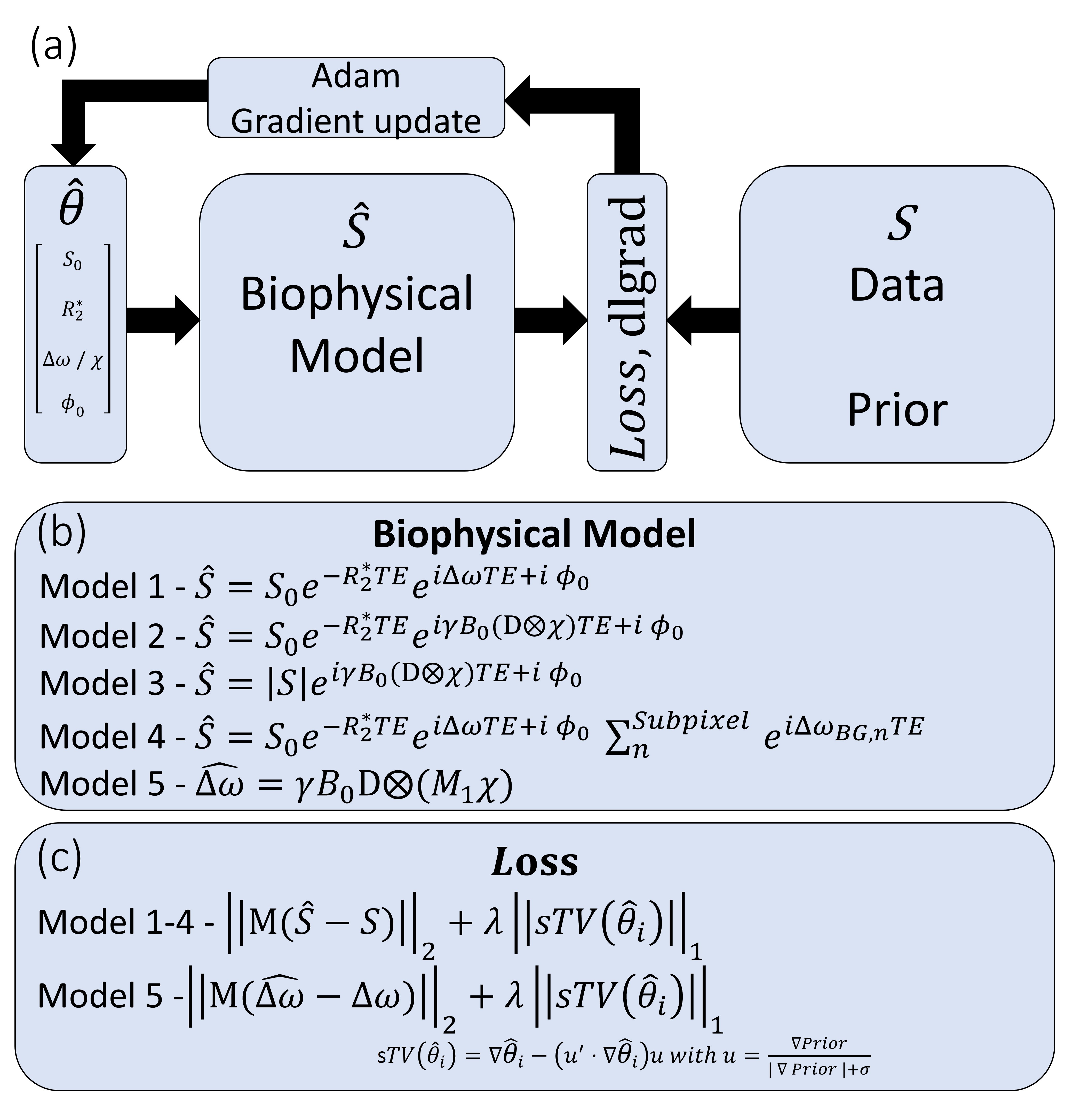
Figure 1a shows the framework used where only the loss-function and the Forward Model are defined. In practice $$$ S(r,TE) $$$ is the concatenation of the real and imaginary components of the 3D multi-echo signal which are compared to the predicted signal $$$ \hat S (r,TE) $$$. Structured total variation (sTV) was employed as regularization in our implementation, as this has been shown to lend well to multi-contrast imaging (5). The forward model is defined as a succession of matrix operations that are differentiable (Fig. 1b shows various models used), and transforms $$$ \theta $$$ (normalized quantitative parameters by $$$weights$$$) into signal.

To demonstrate this methodology, in silico head phantoms were used:

– QSM Challenge 2.0 dataset ($$$ B_0 = 7T$$$, res=1mm, $$$TE_1/ \Delta TE /nTE = 4/8ms/4$$$) and evaluation framework (6) were used to fine-tune optimization parameters (learning rate and $$$ weights $$$ - kept unchanged throughout the abstract), and to benchmark the performance of the QSM reconstruction pipeline: joint $$$R2* \chi$$$ (model 2) and $$$ \chi $$$ alone (model 3); prior based on $$$ S_0$$$, $$$ R_2^*$$$ and $$$ S_0 R_2^*$$$; using L1 or L2 regularization.

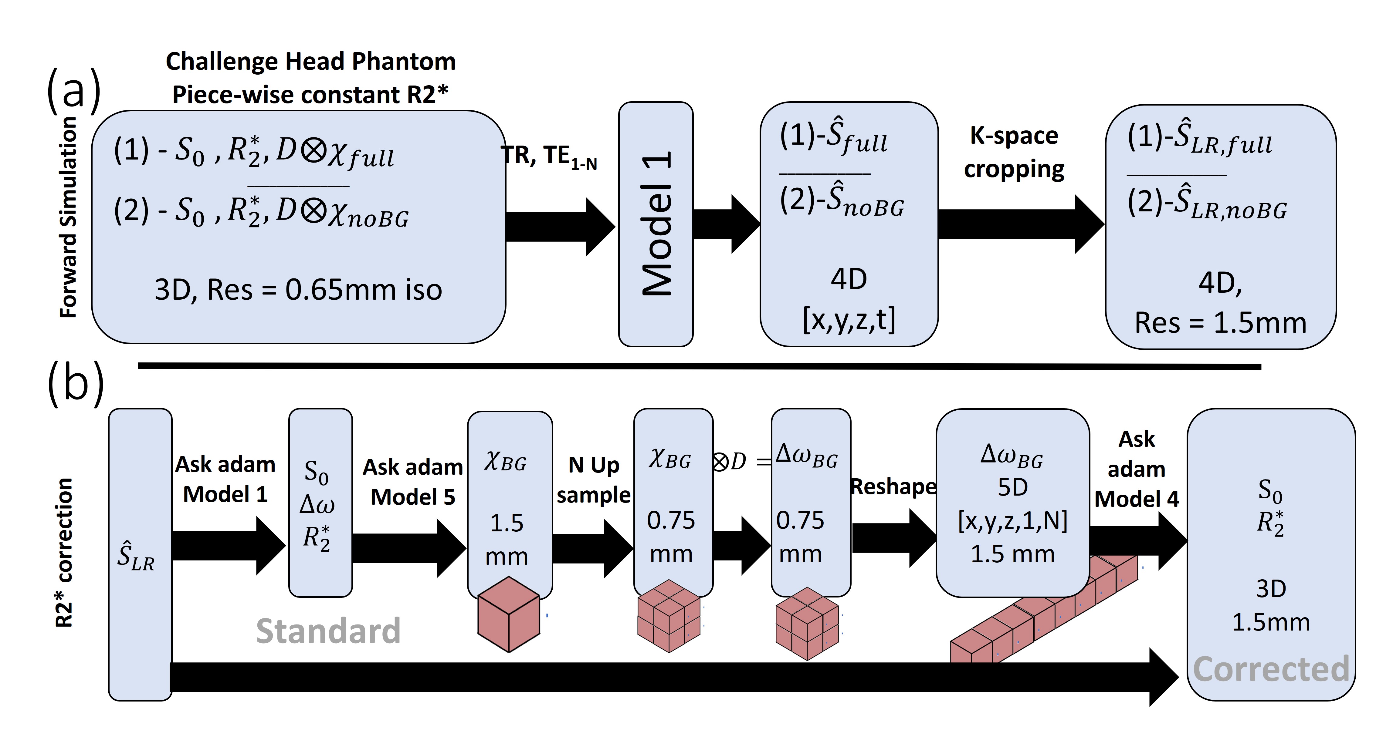
- A variation of the QSM Challenge 2.0 head model (7) where the $$$ R_2^*$$$ of the various tissues were piece-wise constant (one value per tissue type) was used to simulate signal (Fig. 2a) to evaluate the ability to compute R2* maps free of through-slice dephasing artifacts (using the methodology described in Fig.2b). The forward simulations were aimed at emphasizing thes effects ($$$ B_0 = 7T$$$, res=1.5mm, $$$TE_1/ \Delta TE /nTE = 4/8ms/5$$$).

Finally, the networks were tested on 2 heathy volunteer datasets acquired on a 3T scanner (Siemens, Erlangen):

-3DGRE TR/TE1/ΔTE/nTE=44/4/8ms/9, α=[20]°, with transverse slice orientation, FOV=185x2230x141mm³, res=0.8mm iso, α=[20]°, R=3 PF=7/8, TA=10min

-3DGRE TR/TE1/ΔTE/nTE=55/2.68/3.95ms/13, α=[20]°, with sagittal slice orientation, FOV=168x222x240mm³, res=1.5mm iso., R_CAIPI=5, TA=4min

All computations were performed using a Tesla A100 40GB GPU core using Matlab2021b.

Results

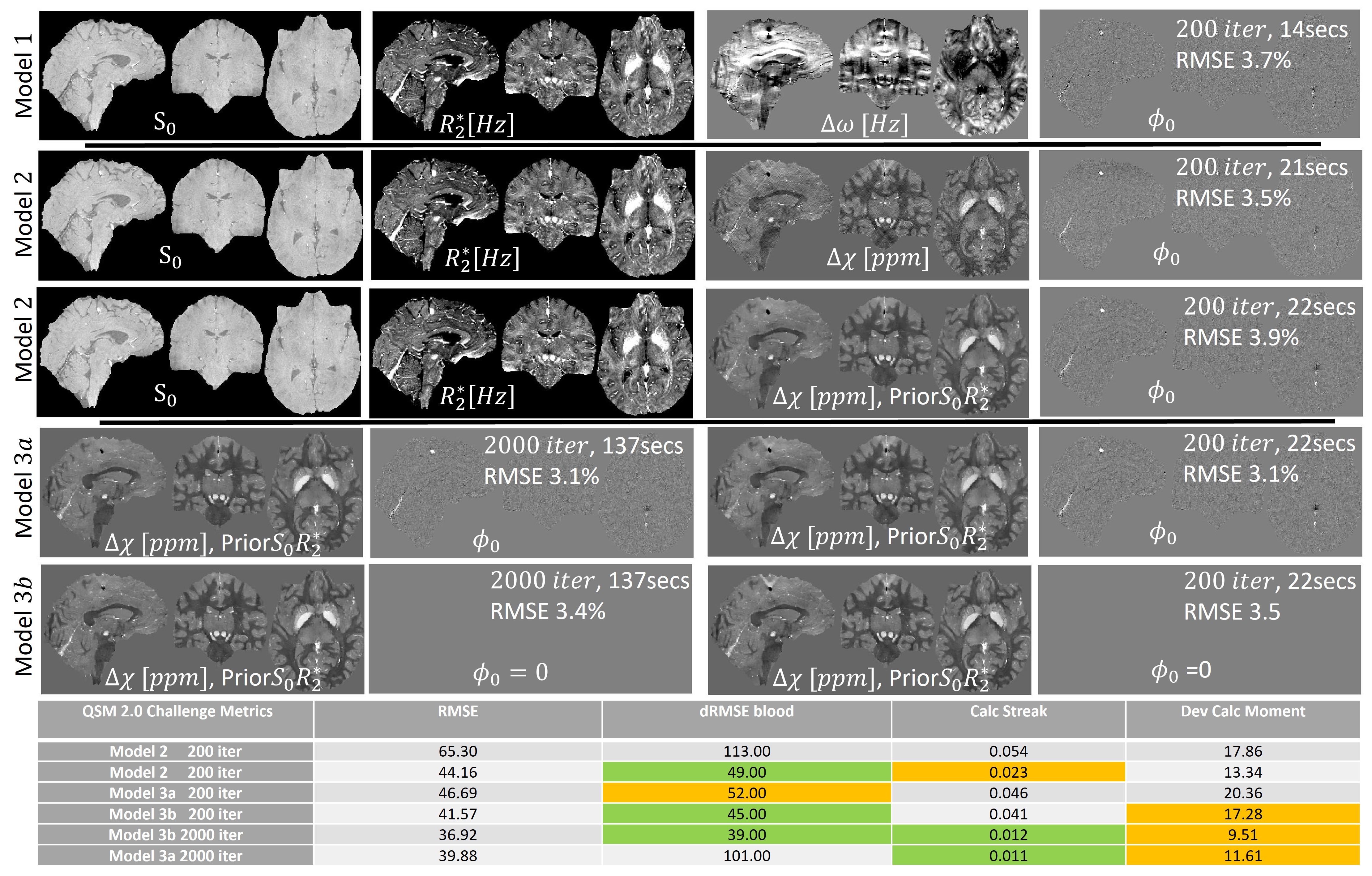
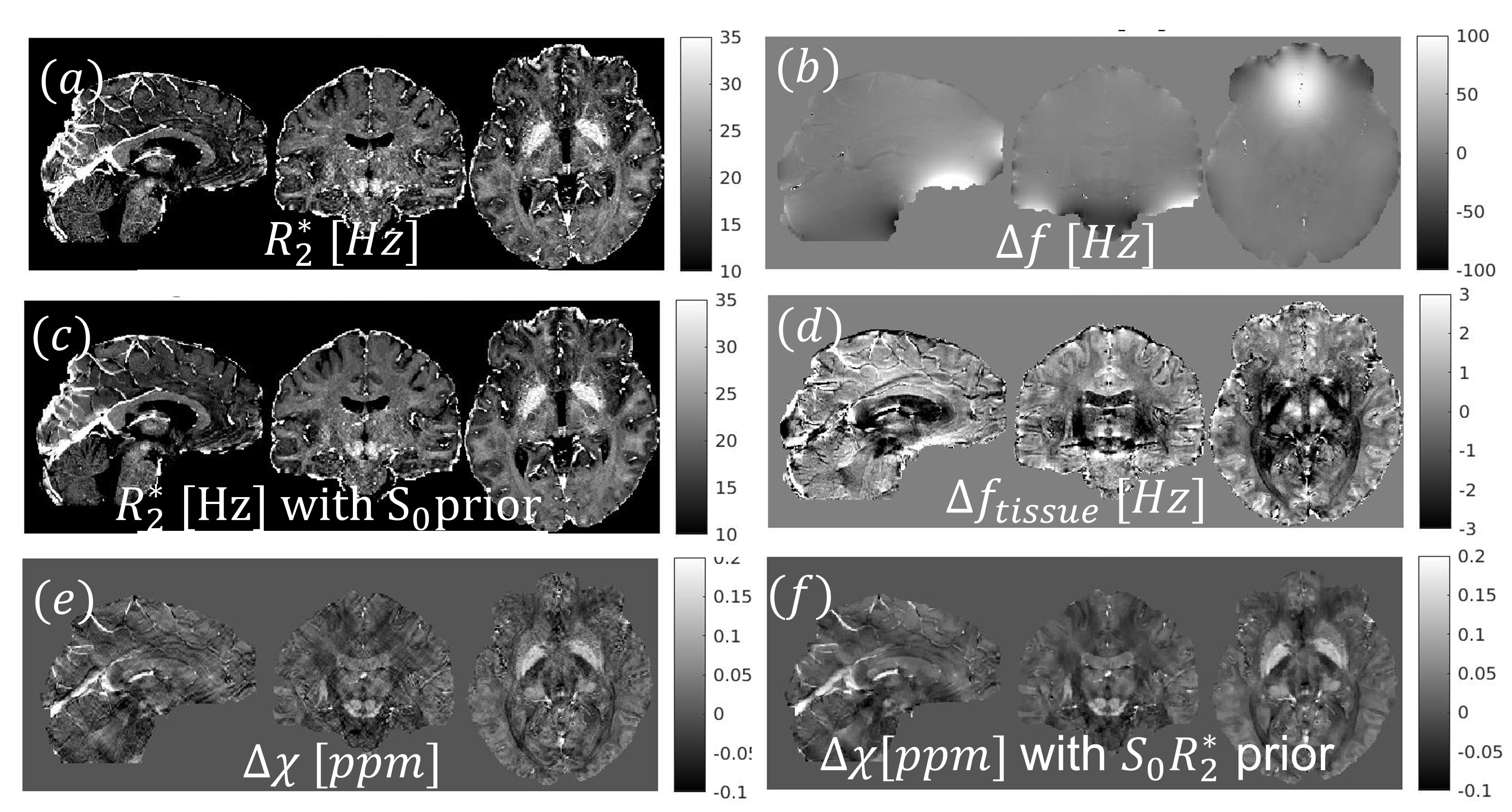
Figure 3 shows the ability to obtain high-quality $$$\chi$$$ maps even in the presence of strong susceptibility sources as calcifications. The non-exhaustive quantitative evaluation showed the L1 regularization based on the sTV having as prior the product of $$$ S0*R2*$$$ resulted in the lowest RMSE, streaking artifacts and calcification moment. Although no large improvements are observed in the data fidelity term after 100 iterations (~10 secs), increasing the iterations to 2000 resulted in improved metrics (see Table in Fig. 3) and reduced artifacts.

This approach was translated to high-resolution in-vivo R2* (and its regularization, Fig 4a and 4.c). It can also be used for all QSM steps: field mapping (Fig. 4b), background field removal (4d), and QSM mapping (4e-f), with all steps performed in <1min.

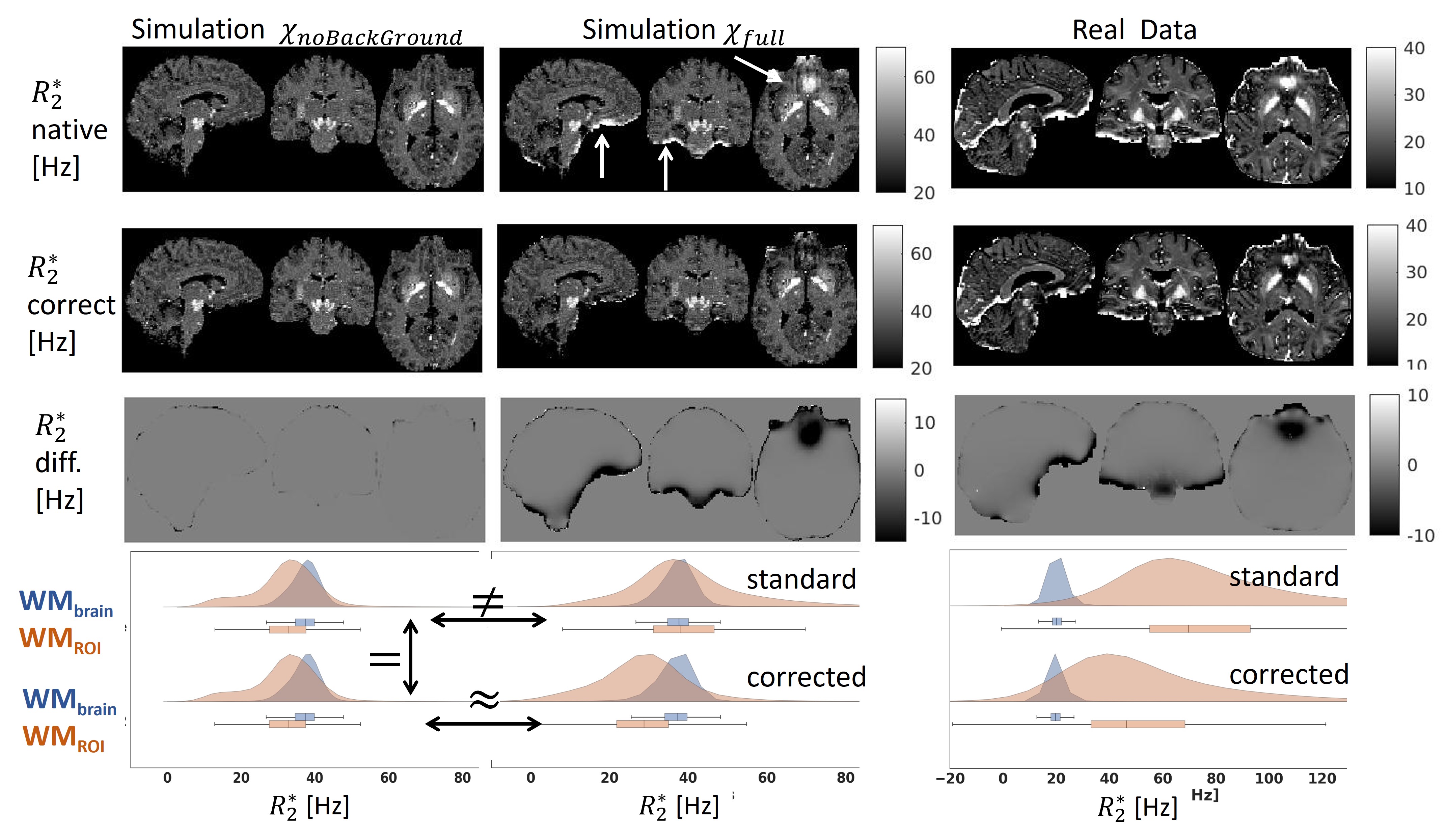
Figure 5 shows the ability of using QSM derived susceptibility distributions to correct for macroscopic intra-voxel dephasing, both in realistic simulations (middle column) and in-vivo data.

Conclusions and Future Work

This framework requires little expertise defining the optimization problem and is flexible. Without adapting the learning rate or weights used to balance different quantitative parameters, it performed parameter fitting at 7T (simulation data), 3T (in vivo data), with resolutions from 0.8 to 1.5mm isotropic and number of echoes from 4 to 13.

In the QSM challenge data, it did not outperform the winning algorithms in nRMSE: effectively solving a quasi-identical gradient descent to FANSI or mcTFI (2,8) and for simplicity we performed a single pass approach. Yet, it won of obtained top 5 on other metrics (green and orange labels in Fig3 Table) that dealt with low SNR (blood RMSE, quantification of calcification moment and streaking artifacts in surrounding the calcification).

The ability to reduce intravoxel dephasing was demonstrated close to air-tissue interfaces, yet it should be equally possible to reduce blooming artifacts surrounding veins by performing the susceptibility mapping prior to the up-sampling step in Fig.2b. Future work will be devoted to using this framework to address water-fat separation and arterial blood displacement in the readout direction in multi-echo acquisitions.

Acknowledgements

No acknowledgement found.