Synopsis

Keywords: Susceptibility, Quantitative Susceptibility mapping

The inversion of tissue magnetic susceptibility from a single-orientation phase measurement is an ill-posed problem. In this work, we propose a novel learning-based constrained reconstruction to integrate the jointly learned tissue field and susceptibility priors with the physics-based dipole inversion formalism such that the non-Gaussian model biased caused by the substantial errors in the estimated tissue field and the streaking artifacts in the tissue susceptibility can be effectively reduced. An efficient solver was also developed to solve the optimization problem. We demonstrated the superior performance of the proposed method over the state-of-the-art dipole inversion method using in vivo datasets.

Introduction

The calculation of tissue magnetic susceptibility from the background-removed, unwrapped local field is an ill-posed inverse problem due to the zero-valued cone surface of the dipole kernel in its Fourier domain. A practical desired approach is to generate tissue susceptibility from a single-orientation gradient-echo measurement, where hand-crafted spatial regularizations^1,2 are often used to suppress the streaking artifacts. However, these methods can lead to prior-dependent shadowing and artifacts, resulting in biased or underdetermined susceptibility values. Recently, deep-learning-based methods have shown significant promise in producing high-quality susceptibility maps by training an end-to-end mapping from the estimated tissue field to the desired susceptibility, including the use of a generic network structure^3-5 or a physics-informed unrolled network architecture^6,7. These data-driven approaches often strongly depend on the quality of training datasets and may be subject to instability issues of deep neural networks. In this study, we proposed a new learning-based constrained reconstruction to integrate the jointly learned tissue field and susceptibility priors with the physics-based dipole inversion formalism. The superior performance of the proposed method over the state-of-the-art dipole inversion method was demonstrated using in vivo datasets.

Theory and Methods

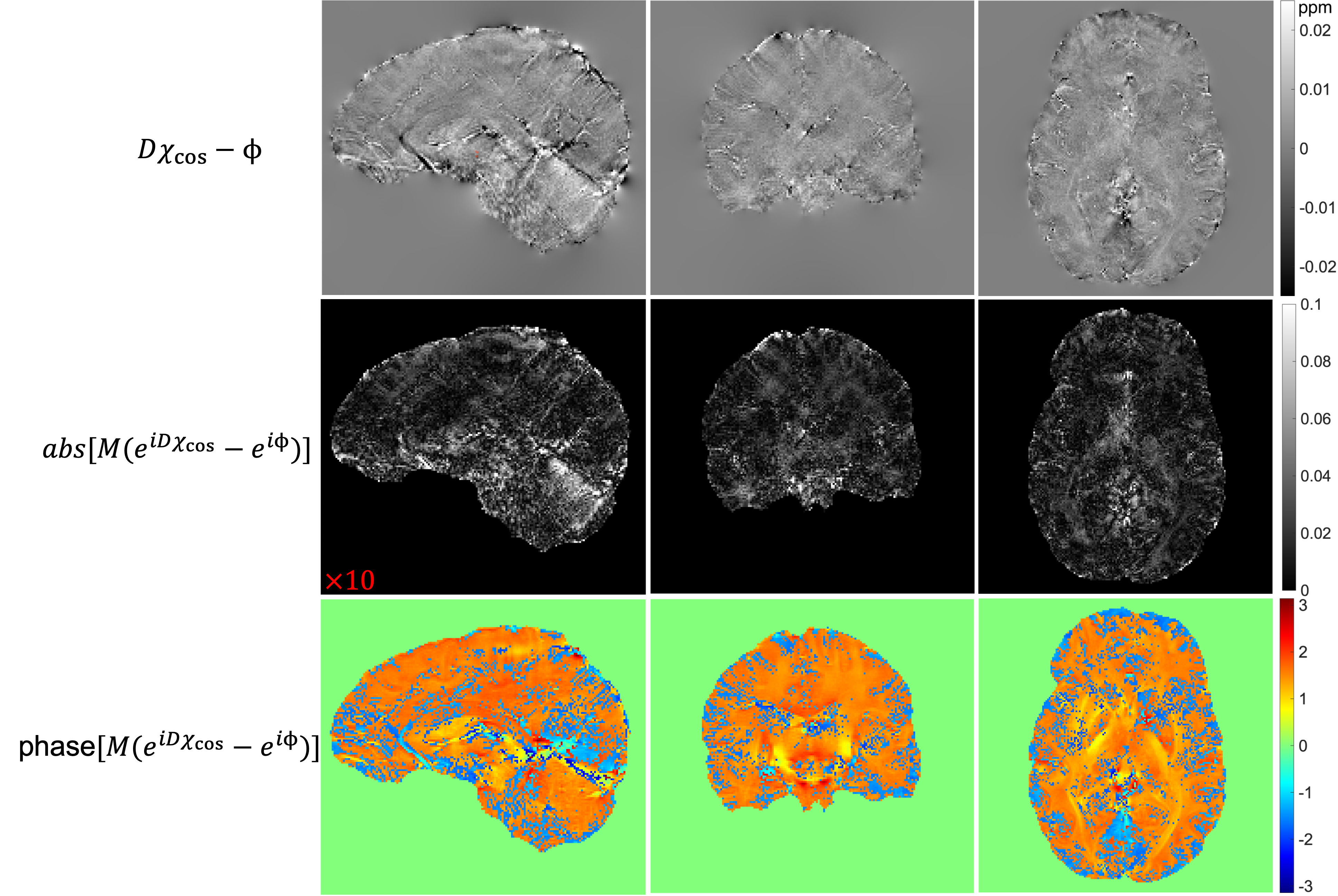
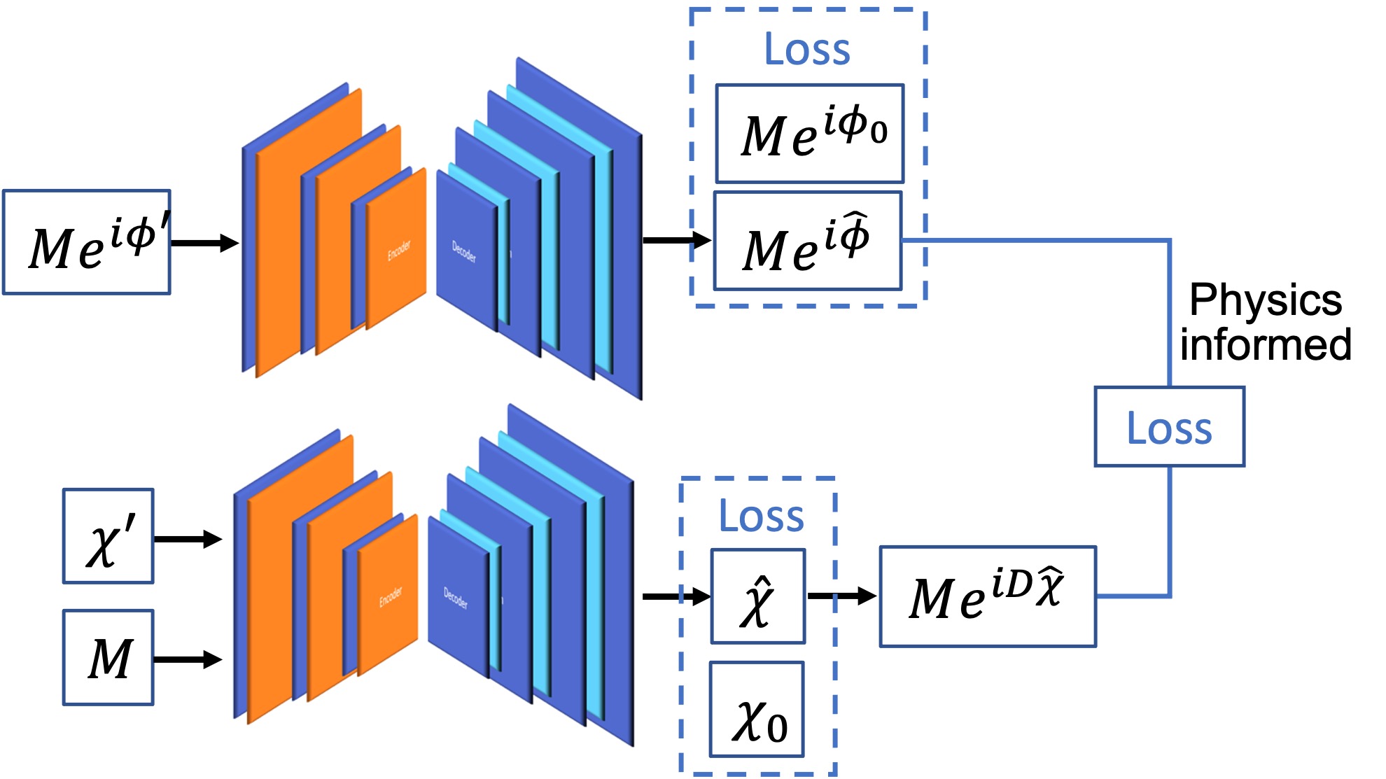
The state-of-the-art physics-based dipole inversion methods used either linear or nonlinear models to represent the relationship between the estimated tissue field and local susceptibility sources. The data-consistency term is usually minimized in the L2 sense, assuming a Gaussian distribution of the model bias. However, there are substantial errors in the estimated tissue field due to SNR and phase-processing issues such that practically the model representation error is usually non-Gaussian. Figure 1 illustrates the non-Gaussian distribution of the errors from linear or nonlinear dipole models using estimated tissue field ($$$\phi$$$) from single-orientation data and the COSMOS⁸ susceptibility (χ_cos) derived from 5-orientation measurements. Moreover, the substantial errors in $$$\phi$$$ can be further enhanced during the poorly-conditioned inversion process. In this work, we propose to mitigate and suppress the errors and artifacts in the tissue field and tissue susceptibility simultaneously by using a new learning-based regularized formulation:$$\underset{\{\chi,\tilde{\phi}\}}{\operatorname{argmin}} \left\| M(e^{iD\chi}-e^{i\tilde{\phi}}) \right\|^2_2+\lambda_1\left\| Me^{i\tilde{\phi}}-g(Me^{i\phi},\theta_g) \right\|^2_2+\lambda_2\left\| \chi-f(\chi,M,\theta_f) \right\|^2_2, (1)$$where $$$M$$$ is the magnitude signal, $$$D$$$ denotes the dipole convolution kernel, $$$\chi$$$ the desired susceptibility distribution. $$$\tilde{\phi}$$$ is an auxiliary field variable with substantially mitigated errors compared to $$$\phi$$$. $$$g(\cdot)$$$ and $$$f(\cdot)$$$ are two "denoising" convolutional deep autoencoders (CDAE) learned from previous database with trainable parameters $$$\theta_g$$$ and $$$\theta_f$$$. The key assumption is that the substantial errors and artifacts in the tissue field and susceptibility do not reside in the latent space and thus can be removed by the learned CDAE. By enforcing the priors that the auxiliary tissue field and the desired susceptibility reside in or be "close to" the low-dimensional manifolds learned by CDAE, both the non-Gaussian model bias in the data consistency and the streaking artifacts in the estimated susceptibility can be well reduced.
1) Joint learning of tissue field and susceptibility priors. We propose to jointly learn the local field and susceptibility priors by leveraging the known physical dipole model. The overall network structure is illustrated in Fig. 2. More specifically, the input tissue phase was estimated using Laplacian phase unwrapping⁹ and VSHARP background field removal¹⁰. The input tissue susceptibility was produced by the nonlinear dipole inversion method⁷. The gold standard COSMOS susceptibility ($$$\chi_{cos}$$$) and its corresponding tissue field ($$$D\chi_{cos}$$$) were paired as labels during training with an L1 loss and a gradient loss to minimize approximation errors, as well as a third physics-informed loss for joint learning.
2) Efficient solver for the regularized optimization problem. We propose to solve Eq.(1) using alternating minimization, which alternates between two sub-problems:$$\underset{\chi}{\operatorname{argmin}} \left\| M(e^{iD\chi}-e^{i\tilde{\phi}}) \right\|^2_2+\lambda_2\left\| \chi-f(\chi,M,\theta_f) \right\|^2_2, (2)$$ $$\underset{\tilde{\phi}}{\operatorname{argmin}} \left\| M(e^{iD\chi}-e^{i\tilde{\phi}}) \right\|^2_2+\lambda_1\left\| Me^{i\tilde{\phi}}-g(Me^{i\phi},\theta_g) \right\|^2_2, (3)$$ To solve Eq.(2), we used the plug-and-play ADMM¹¹, which alternates between a quadratic minimization problem and a "denoising" step using the pre-trained CDAE $$$f(\cdot)$$$. For Eq.(3), the update of $$$\tilde{\phi}$$$ is the weighted average of the outputs of the forward dipole model and the pre-trained CDAE $$$g(\cdot)$$$.

Experiments and Results

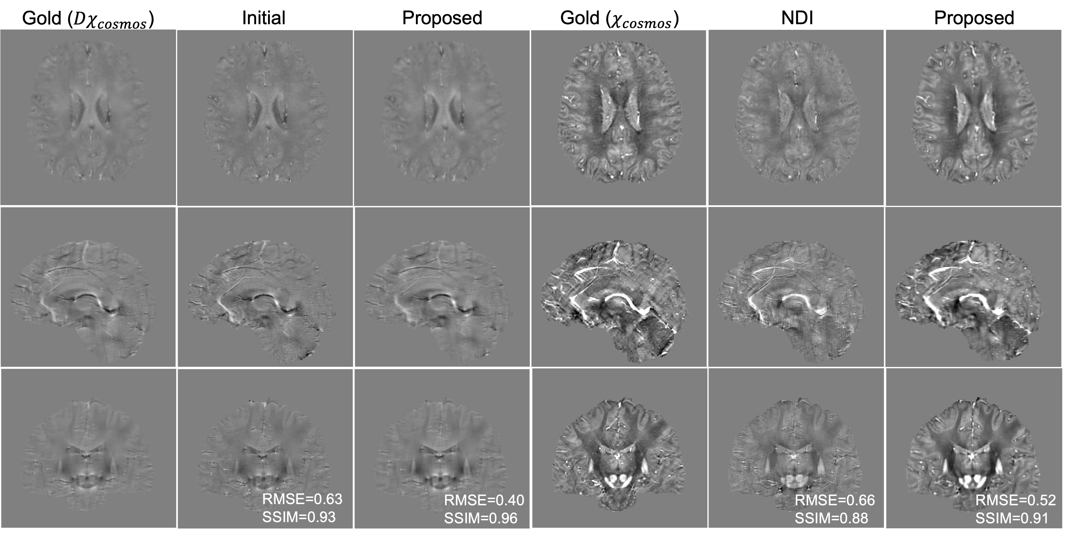
We used the QSMnet+ datasets to train (8 subjects) and validate (4 subjects) the proposed model where the COSMOS susceptibilities were derived from five-orientation 3D GRE scans (matrix size 176×176×160mm³, resolution 1mm isotropic, TE/TR 25/35ms, FA 15°). The network was constructed in Tensorflow 2.0 and trained using stochastic gradient descent with an Adam optimizer for 200 epochs using two NVIDIA RTX A6000 GPUs, taking approximately 54 hours.
We compared our method with the state-of-the-art NDI reconstruction. Results are reported in Fig. 3. As can be seen, the proposed method provides consistently high-quality susceptibility maps in terms of fewer artifacts and better quantitative metrics, and reveals a very similar contrast close to that of COSMOS with visually even higher SNR. The associated tissue field produced by our method also exhibits a "cleaner" appearance with much fewer phase errors compared to the initial estimated ones.

Conclusion

A novel learning-based regularized dipole inversion formulation is proposed to produce high-quality susceptibility maps from single-orientation measurement by taking advantage of the physical dipole model and the jointly learned local field and susceptibility priors.

Acknowledgements

We would like to thank Profs. Jongho Lee and Eun Young Choi for sharing their QSMnet dataset.