Synopsis

Keywords: Microstructure, White Matter

A hollow cylinder fiber model (HCFM) with two orientation-dispersed fiber populations was used to characterize white matter microstructure-based susceptibility effects. The resulting TE-dependent frequency shifts were fitted with a curve function parameterized by a microstructure induced frequency difference (Δf) and bulk susceptibility induced frequency shift (C_f). Local frequency and QSM reconstruction using the fitted C_f versus using weighted echo averaging were compared by a head phantom and in vivo human brain data. Δf provided a useful contrast to illustrate the underlying white matter microstructure and C_f helped to improve the quantification accuracy of tissue magnetic susceptibility using QSM.

Introduction

Previous studies reported the effects of white matter (WM) microstructure on gradient-echo-based local frequency shifts^1-3. Such effects cannot be explained by quantitative susceptibility mapping (QSM)⁴ or susceptibility tensor imaging (STI)⁵, and would introduce artifacts and potentially under- or over-estimated tissue magnetic susceptibilities. Therefore, accurate characterization of the microstructure induced frequency shifts is important for improved quantification of tissue susceptibility and assessment of the underlying tissue microstructures. Here, we investigated the WM microstructure-induced frequency shift in voxels using a hollow cylinder fiber model (HCFM) with two orientation-dispersed fiber populations. In addition, we performed TE-dependent frequency fitting method to separate the time-dependent microstructure-induced frequency from the time-independent bulk susceptibility induced frequency shift for QSM. Reconstruction performances were evaluated using a head phantom and in vivo data.

Methods

The relationship between the microstructure-induced frequency difference Δf and TE-dependent frequency f can be represented as Eq. (1) ²:
$$f(TE) = \Delta f\left(\frac{exp\left(-[R_{2,my}^*-R_{2,(ax\&ex)}^*]\cdot TE\right)}{MVF\left(exp\left(-[R_{2,my}^*-R_{2,(ax\&ex)}^*]\cdot TE\right)-1\right)+1}\right)+C_{f} \qquad (1)$$
where MWF is the myelin water fraction; $$$R_{2,my}^*$$$ and $$$ R_{2,(ax\&ex)}^*$$$ are relaxation rates in the myelin and axon/extra-cellular compartments, respectively. $$$C_{f}$$$ is the time-independent frequency shift induced by bulk magnetic susceptibility.

Multi-shell diffusion weighted (DW) EPI MRI scans (voxel size = 1.5×1.5×1.5 mm³, TR/TE = 3350/86 ms, 7, 46, 46 gradient directions for b = 0, 1500, 3000 s/mm²) were acquired on a 3T Philips Ingenia RX scanner. For $$$\Delta f$$$ and QSM, a 3D multi-echo GRE sequence was applied with TR/TE₁/∆TE = 77/2.8/2.2 ms, 15 unipolar echoes, voxel size = 1×1×1 mm³, FOV = 220×192×100 mm³ at 7T.

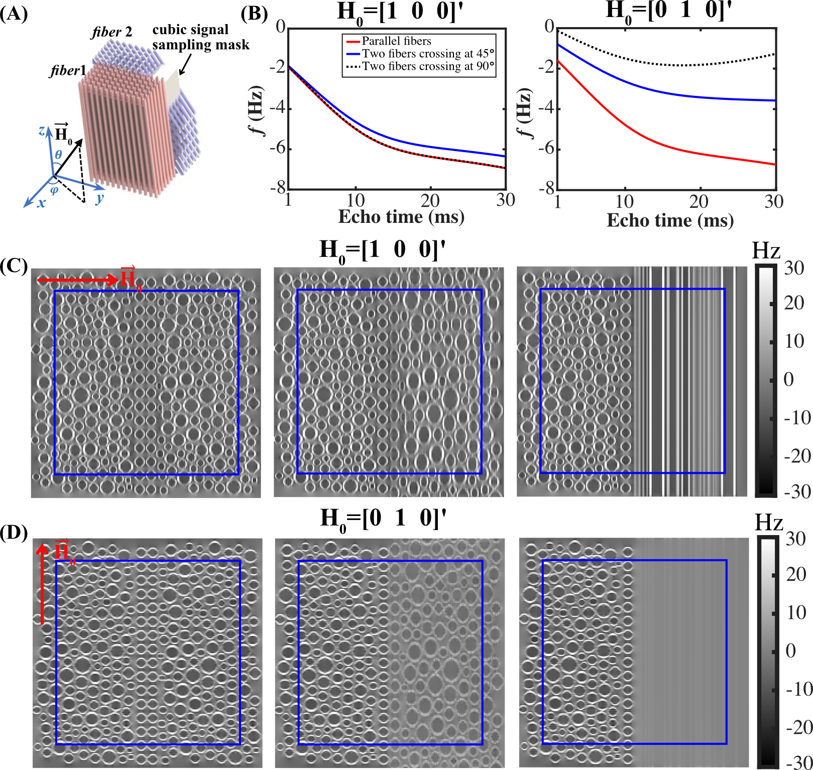
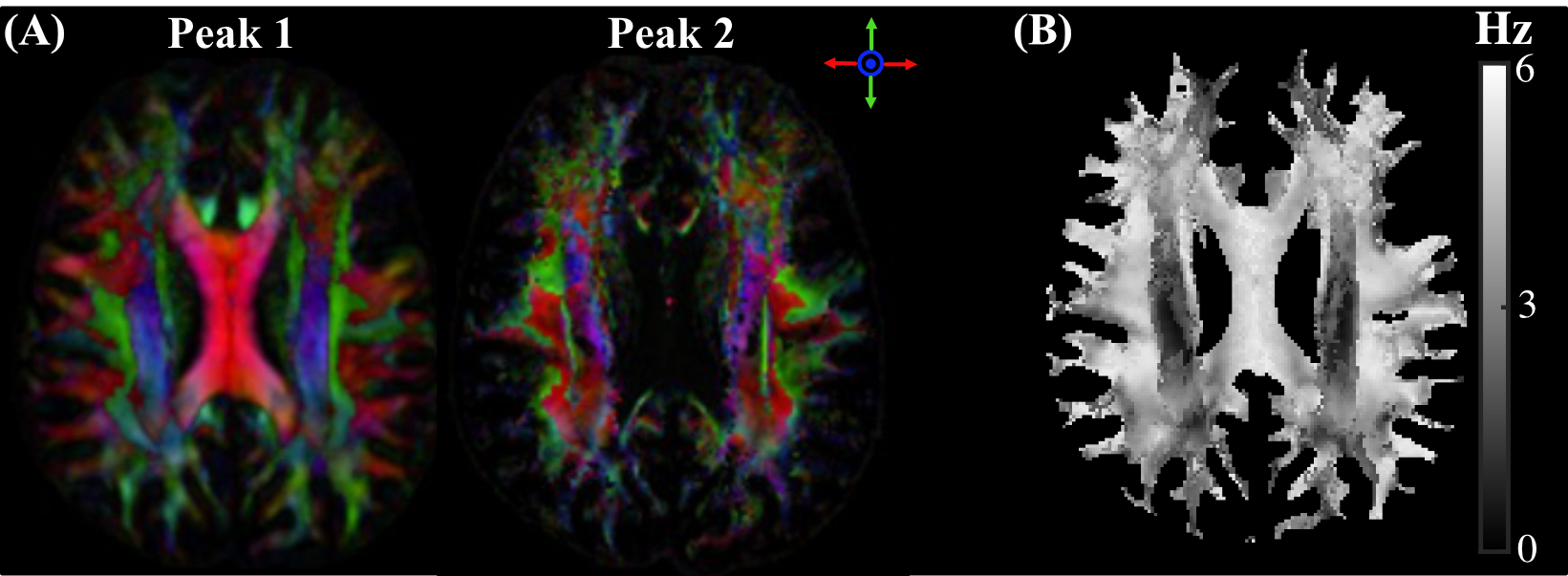
A HCFM^1,2 with two fiber populations was used to simulate the field perturbation inside WM voxels. Each model has a 200×200×200 sub-voxel grid, with 156 and 161 cylinders simulated for the two fiber populations, respectively (Fig. 1a). Within the coordinate system aligned with fiber 1, fiber 2 direction = $$$\begin{bmatrix}0 & sin\alpha&cos\alpha \end{bmatrix}'$$$ and $$$\widehat{H}_{0}=\begin{bmatrix}sin\theta cos\varphi & sin\theta sin\varphi&cos\theta \end{bmatrix}'$$$ , where $$$\theta=\beta_{1}$$$ and $$$\varphi=sin^{-1}\left(\frac{cos\beta_{2}-cos\alpha cos\beta_{1}}{sin\alpha sin\beta_{1}}\right)$$$. Peaks of the fiber orientation distribution function (ODF) estimated from diffusion MRI⁶ were used to determine the angles $$$\alpha$$$ as well as the angles $$$\beta_{1}$$$ and $$$\beta_{2}$$$ between B₀ and each fiber population, respectively. Crossing fiber voxels were assigned when the amplitude of ODF peak 2 was greater than 30% of peak 1. $$$\alpha$$$ was further divided into 19 groups with 5° span for each group.

A head phantom was generated to simulate MRI signal evolution with frequency contributions from bulk isotropic and anisotropic magnetic susceptibility and WM microstructures. The isotropic susceptibility component was assigned according to brain atlas and literature values.⁷ The anisotropic susceptibility was added in WM and modulated by fiber orientation dispersion estimated using NODDI⁸. Gradient echo signal was calculated using $$$S=S_{0}e^{-TE\cdot R_2^*}\cdot(1-e^{-TR\cdot R_{1}})\cdot\frac{sin\left(FA\right)}{1-cos\left(FA\right)\cdot e^{-TR\cdot R_{1}}}\cdot e^{i\left(2\pi\cdot TE\cdot \Delta f +\varphi_{0} \right)}$$$ , where $$$\Delta f=\Delta f_{macro}+\Delta f_{micro}$$$ . $$$\Delta f_{macro}$$$ was calculated using the STI forward model⁵ and $$$\Delta f_{micro} = \Delta f\left(\frac{exp\left(-[R_{2,my}^*-R_{2,(ax\&ex)}^*]\cdot TE\right)}{MVF\left(exp\left(-[R_{2,my}^*-R_{2,(ax\&ex)}^*]\cdot TE\right)-1\right)+1}\right)$$$ from multi-fiber HCFM.

f(TE) were estimated using temporal ROMEO phase unwrapping⁹ with MCPC-3D¹⁰ to remove $$$\varphi_{0}$$$ and LBV¹¹ for background removal. $$$\Delta f$$$and $$$C_{f}$$$ were then reconstructed by weighted least square fitting of Eq. (1) with weights of $$$\omega_{n} = \frac{TE_{n}\cdot e^{-\frac{TE_{n}}{T_2^*}}}{\sum_{n=1}^N TE_{n}\cdot e^{-\frac{TE_{n}}{T_2^*}}}$$$. QSM images were reconstructed by iLSQR¹² from $$$C_{f}$$$ as compared to local field calculated using weighted echo averaging.

Results and Discussion

Figure 1(A) shows the HCFM with two fiber populations. Fig. 1(B) shows the signal frequency over TEs for $$$\widehat{H}_{0}$$$ of $$$\begin{bmatrix}1 & 0& 0 \end{bmatrix}'$$$ and $$$\begin{bmatrix}0 & 1& 0 \end{bmatrix}'$$$ in parallel fibers, two fiber populations crossing at 45° and 90°. Fig. 1(C&D) show the corresponding simulated field perturbation.

Fig.2 shows color maps of the first and second ODF peak and the simulated $$$\Delta f$$$ using Eq. (1).

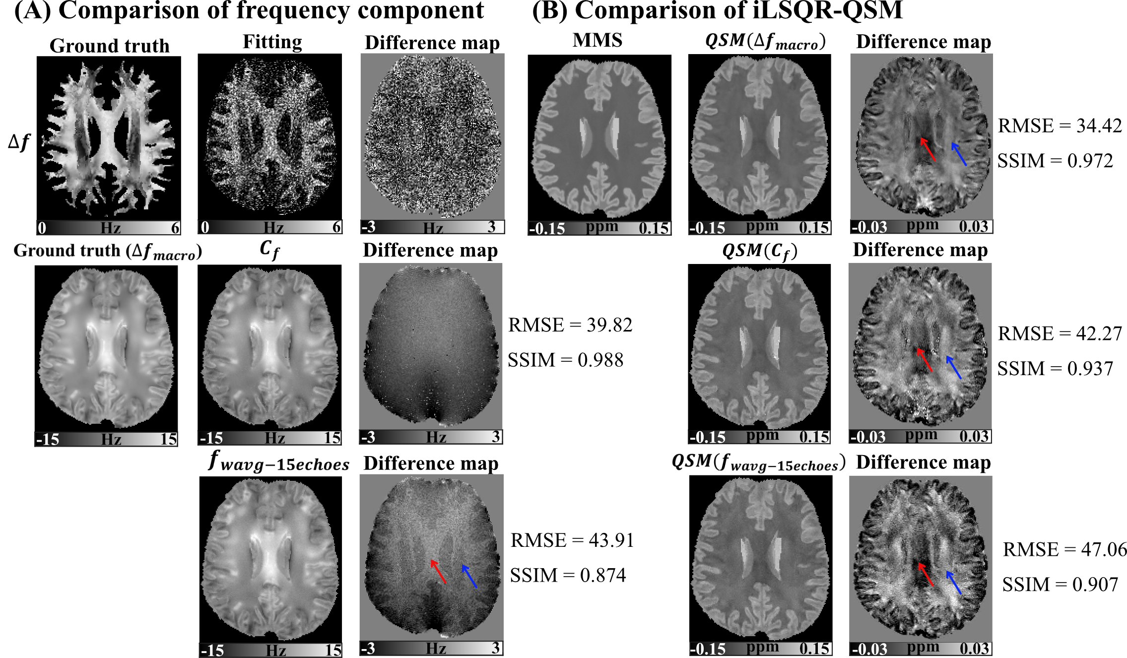
For head phantom, though noisier, the fitted $$$\Delta f$$$ shows the same anatomical features and orientation dependence as compared to the ground truth. Without considering the microstructure-induced frequency shift, larger error was observed in weighted echo averaging ($$$f_{wavg-15echoes}$$$) with higher RMSE and lower SSIM (Fig. 3(A)). The difference between $$$QSM(\Delta f_{macro})$$$ and mean magnetic susceptibility (MMS) shows different error patterns for differently orientated fibers (red and blue arrow) due to the unaccounted susceptibility anisotropy effect in QSM deconvolution. $$$QSM(C_{f})$$$ outperforms $$$QSM(f_{wavg-15echoes})$$$ with lower RMSE and higher SSIM, especially in CC (red arrow) and superior region of CR (blue arrow) (Fig. 3(B)).

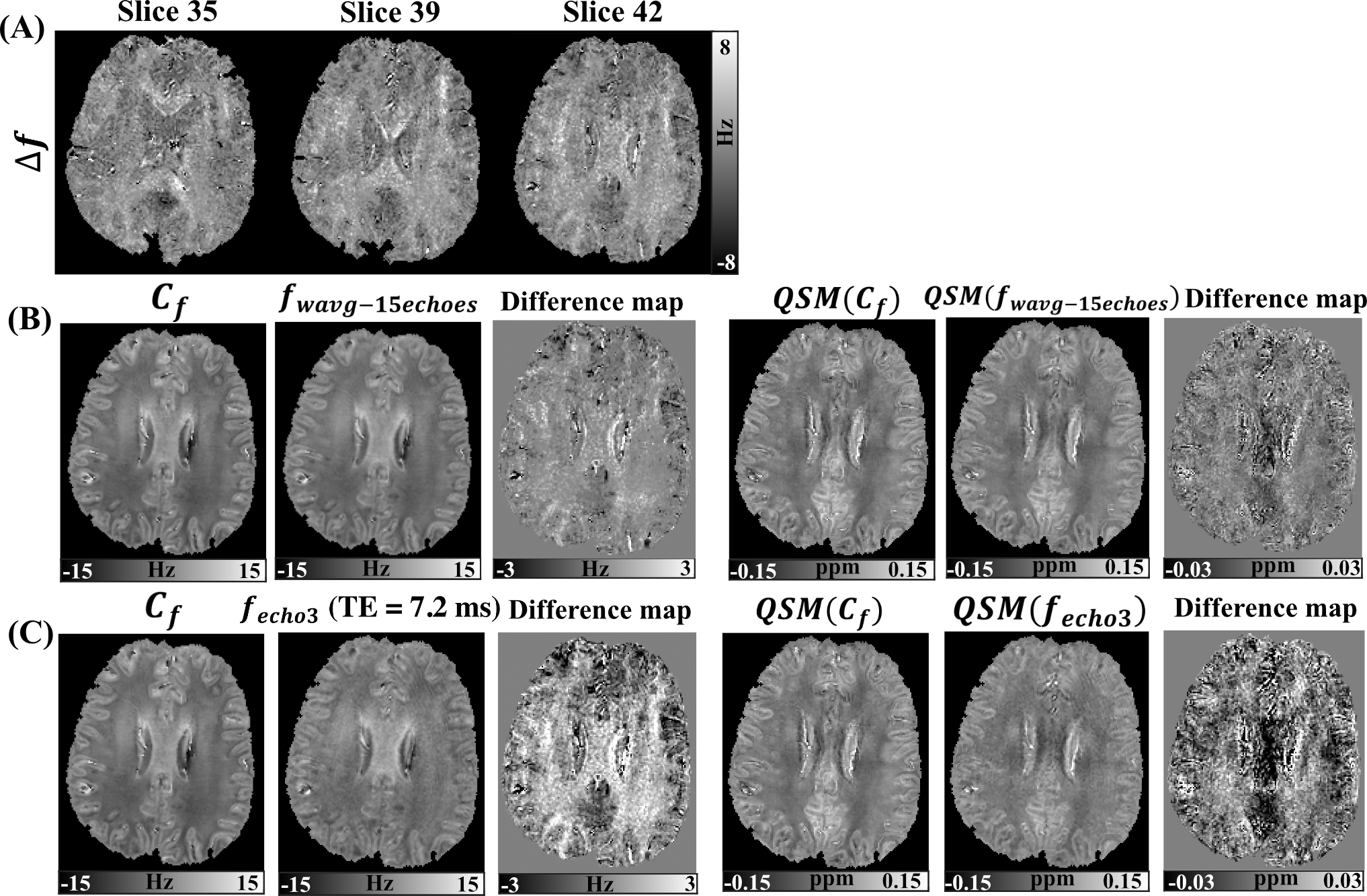
Fig. 4 (A) shows representative slices for in vivo fitted $$$\Delta f$$$. Fig. 4 (B) compares the $$$C_{f}$$$ and $$$f_{wavg-15echoes}$$$. The microstructure-induced frequency residuals are shown in the difference map and propagate to the final QSM. Fig. 4 (C) compares the $$$C_{f}$$$ and $$$f_{echo3}$$$ estimated at the third echo and the corresponding QSM maps. Differences in comparison to the fitted $$$C_{f}$$$ show that $$$f_{echo3}$$$ gives larger microstructure-induced frequency residuals (>2 Hz) than $$$f_{wavg-15echoes}$$$ (~1 Hz) which also leads to larger differences in QSM.

Conclusion

The HCFM with two fiber populations can well characterize microstructure-induced frequency shifts. Such microstructure effects are expected to bias the estimation of tissue magnetic susceptibility using QSM. A bio-physical model-based TE-dependent frequency fitting method may help obtain a useful contrast related to the tissue microstructure ($$$\Delta f$$$) and help improve the quantification accuracy of bulk magnetic susceptibility induced frequency shift ($$$C_{f}$$$) and the corresponding QSM.

Acknowledgements

This work was supported by NIBIB (P41EB031771).