Synopsis

Keywords: Motion Correction, Brain

Rigid head motion, which is a challenging problem in itself, is further accompanied by field variations as the object moves in an inhomogeneous background field, and because pose changes lead to varying susceptibility-induced fields. In contrast to external sensors like optical cameras, navigators are naturally sensitive to field variations. We propose a fast, scan-integrated calibration method to sensitize the 3D orbital navigators to rigid motion and 1st order shim fields. The obtained motion and field parameters are used to correct the scan geometry and shim settings in real-time. The performance is evaluated in phantom and in-vivo studies.

Introduction

Head motion is one of the major challenges in MRI requiring scans to be repeated and limiting the effective image resolution [1]. This problem has been addressed by prospective [1] and retrospective [2] rigid motion correction methods. In addition to the rigid alignment, subject motion dynamically interacts with the MR fields during a scan causing field changes in the head frame, esp. in high-field, high-resolution imaging situations. Real-time shimming and geometry correction with NMR probes [3] have been shown to improve image quality substantially. Also, navigation methods like the cloverleaf [4] have been proposed to achieve real-time geometry and 1st order shim correction, but this method still requires a motion-less 12-s pre-scan and 4.2 ms time per TR. We propose a gradient shim calibration as an extension to the 3D orbital navigator approach [5] that offers high-precision motion and 1st order shim correction, while requiring sub-second scan-integrated pre-scans and 2.3 ms time per TR.

Methods

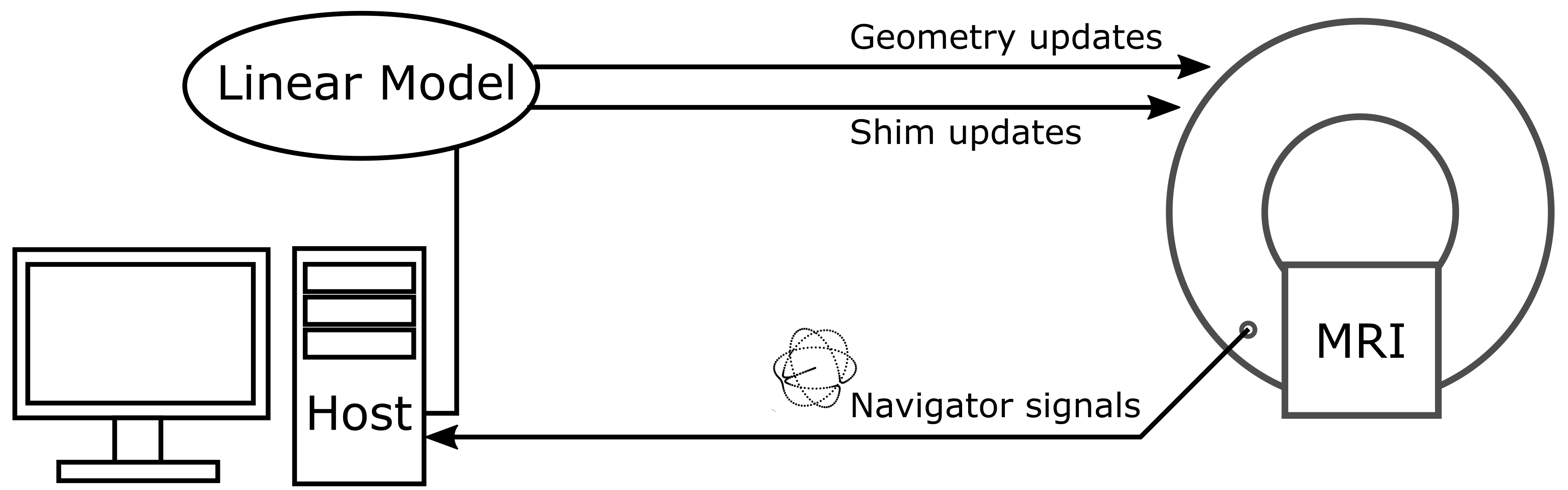
An overview of the real-time pipeline for rigid motion and gradient shim correction is shown in Fig. 1. Navigator signals are acquired every TR and sent to the host computer. Updates for the geometry and shims (up to first order) are estimated for the new navigator using a linear perturbation model. The updated parameters are sent back to the scanner to adjust the scan geometry and shim settings.

The linear perturbation model connects the multi-coil signal difference to the reference navigator $$${\boldsymbol \Delta s}$$$ to the changes in the motion and shim parameters $$${\boldsymbol \Delta p}$$$ via a linear model [6]:

$${\boldsymbol \Delta s} = {\boldsymbol s}_{cur} - {\boldsymbol s}_{ref} = \begin{bmatrix}\frac{\delta {\boldsymbol s}}{\delta \Delta p_1} & ... & \frac{\delta {\boldsymbol s}}{\delta \Delta p_{N_p}}\end{bmatrix} \cdot {\boldsymbol \Delta p}.$$

The columns of the model matrix are the derivates of the signal model with respect to the associated parameter. In this work, $$${\boldsymbol \Delta p}$$$ contains $$${N_p = 11}$$$ parameters, namely 6 rigid, 1 B0 off-resonance, 3 gradient shim and 1 phase offset parameter. The derivatives for rigid shifts, the phase offset and the B0 off-resonance can be derived analytically from one navigator signal vector [6]. Following the idea presented in Ref. [7] for rotations, the derivatives for rotations and gradient shims are determined by a finite difference approach, where additional reference navigators are acquired with 0.5 degree rotations and 5 µT / m shim offsets, respectively. Thus, seven reference navigators are required here.

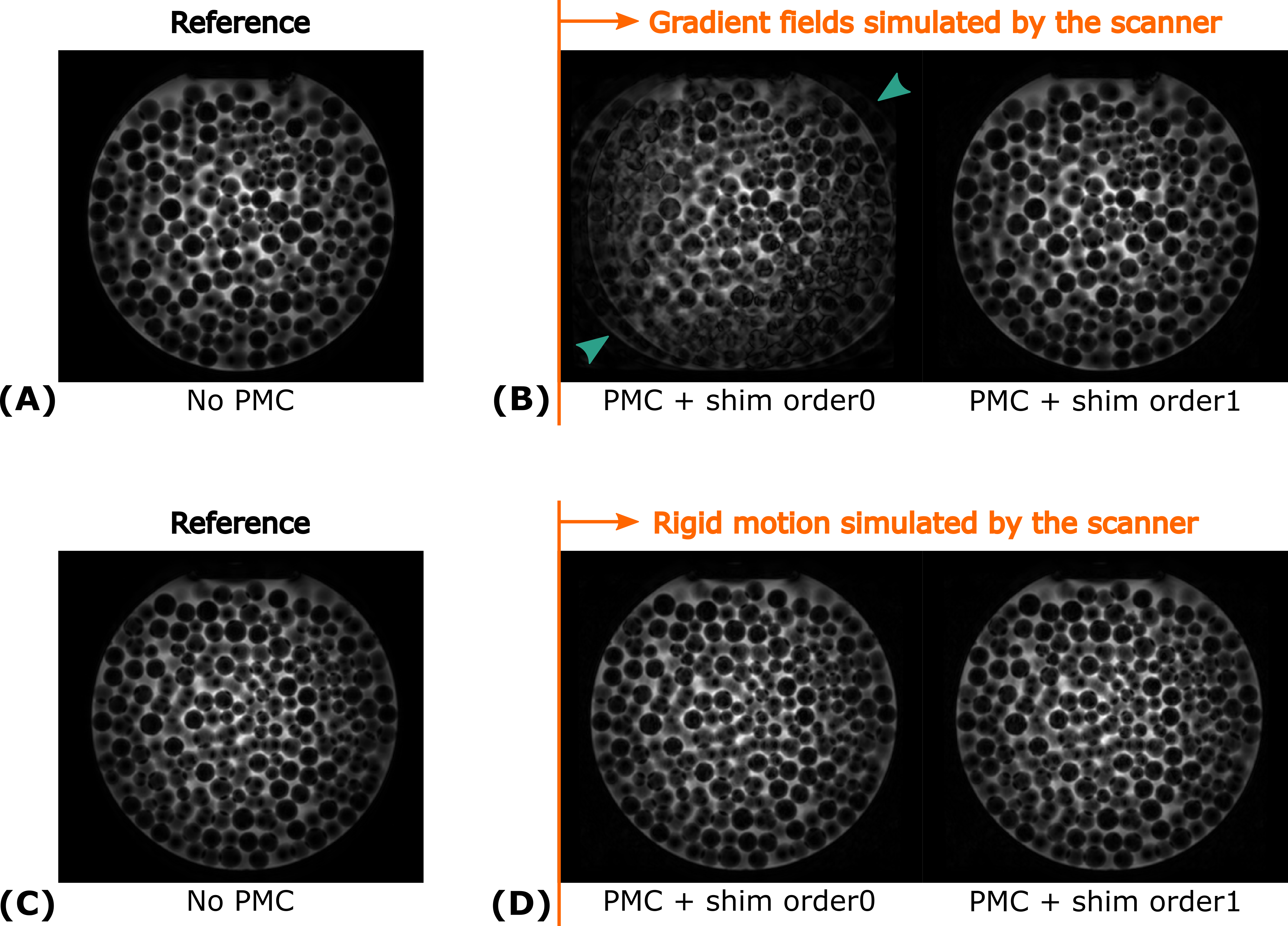
The proposed method, termed ‘PMC + shim order1’, was tested in phantom experiments and in-vivo. Adapting the approach by Buschbeck et al. [8], the correction performance was evaluated by actively disturbing the scan geometry and the gradient shim settings during the scan to analyze the associated step response behavior of the system. The system was disturbed every 100 TRs by either 2 mm, 2 deg, or 10 µT / m shim offsets. For comparison, the scans were repeated with ‘No PMC’, and with PMC and only 0th order shimming, called ‘PMC + shim order0’.

The navigator was inserted into a 3D GRE sequence between the excitation and the imaging readout. The scans were performed on a 7T Philips Scanner (Best, The Netherlands) with a 32-channel coil. Phantom data was acquired at 1 x 1 x 4 mm³ with 18° flip angle, TE = 8.5 ms, TR = 45 ms. In-vivo data was acquired from two subjects at 0.6 x 0.6 x 1.2 mm³ with 3° flip angle, TE = 8 ms, TR = 20 ms, and 4-fold SENSE acceleration (2:09 min). Informed consent from the subjects was attained according to the rules of the institution.

Results

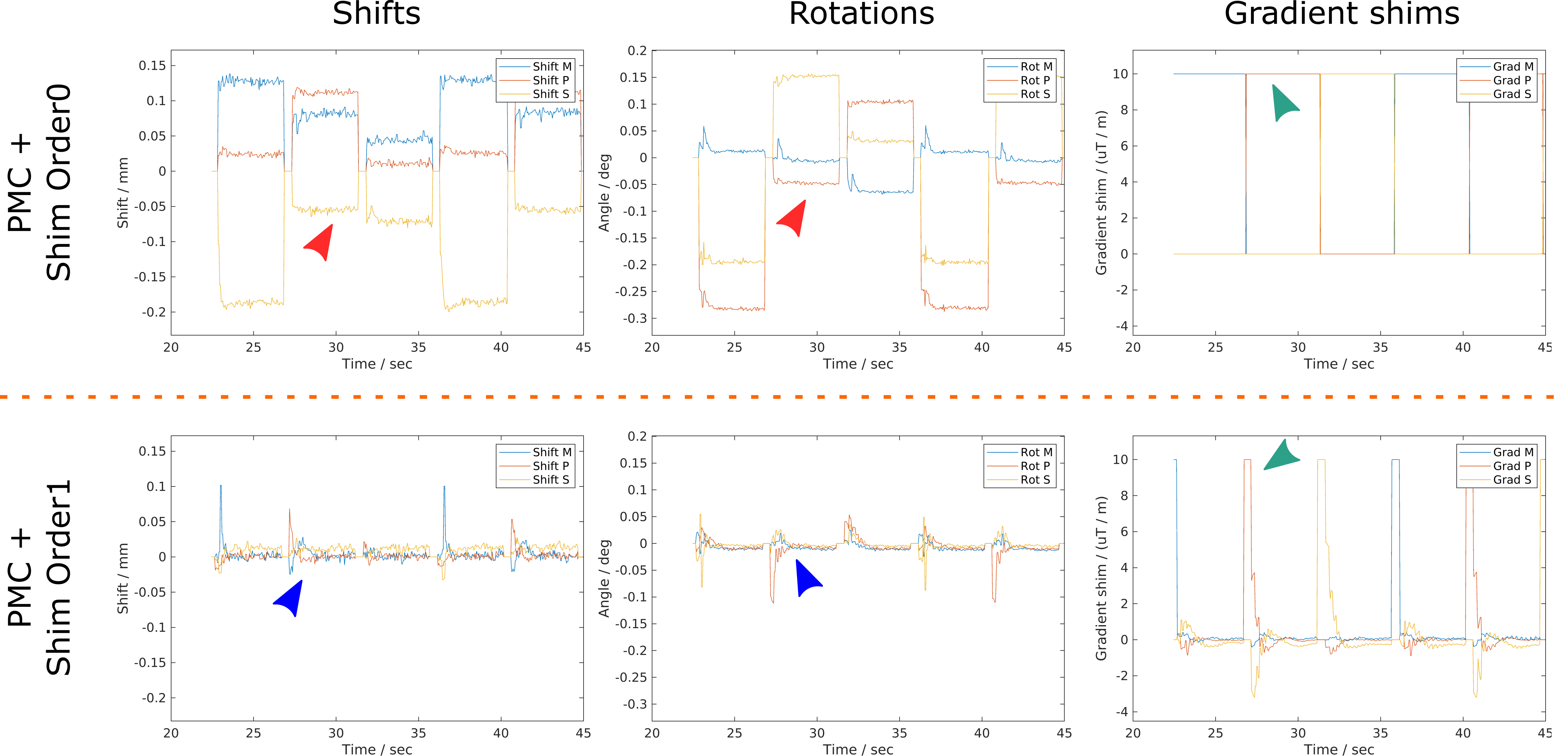
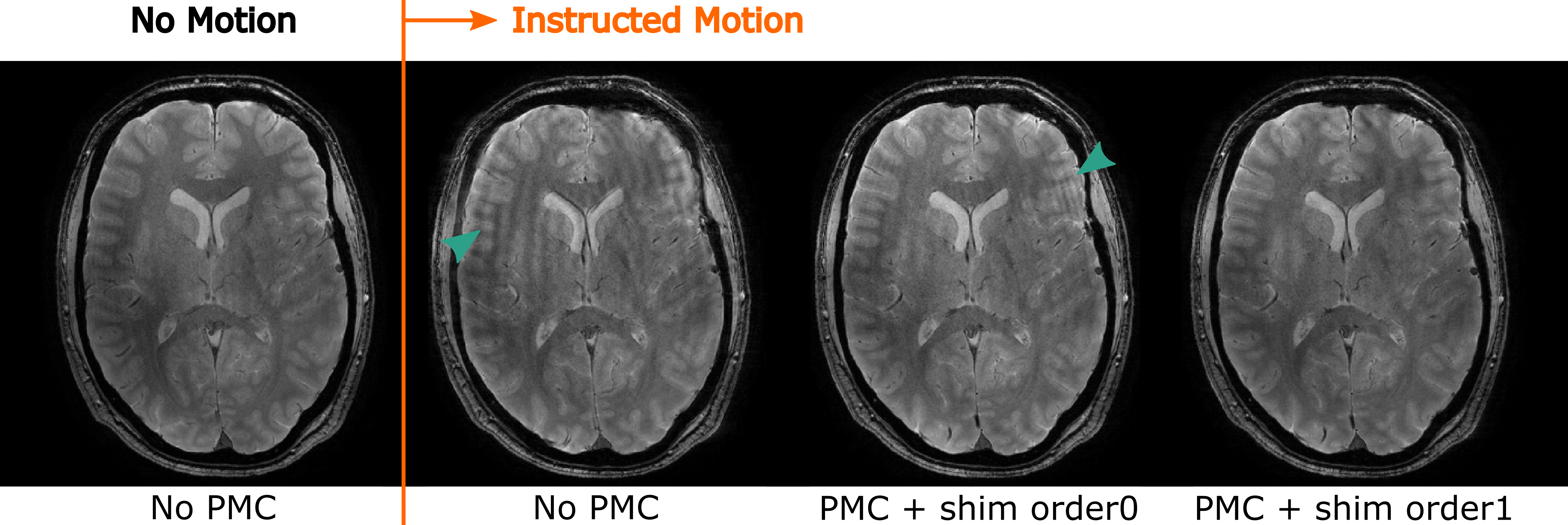
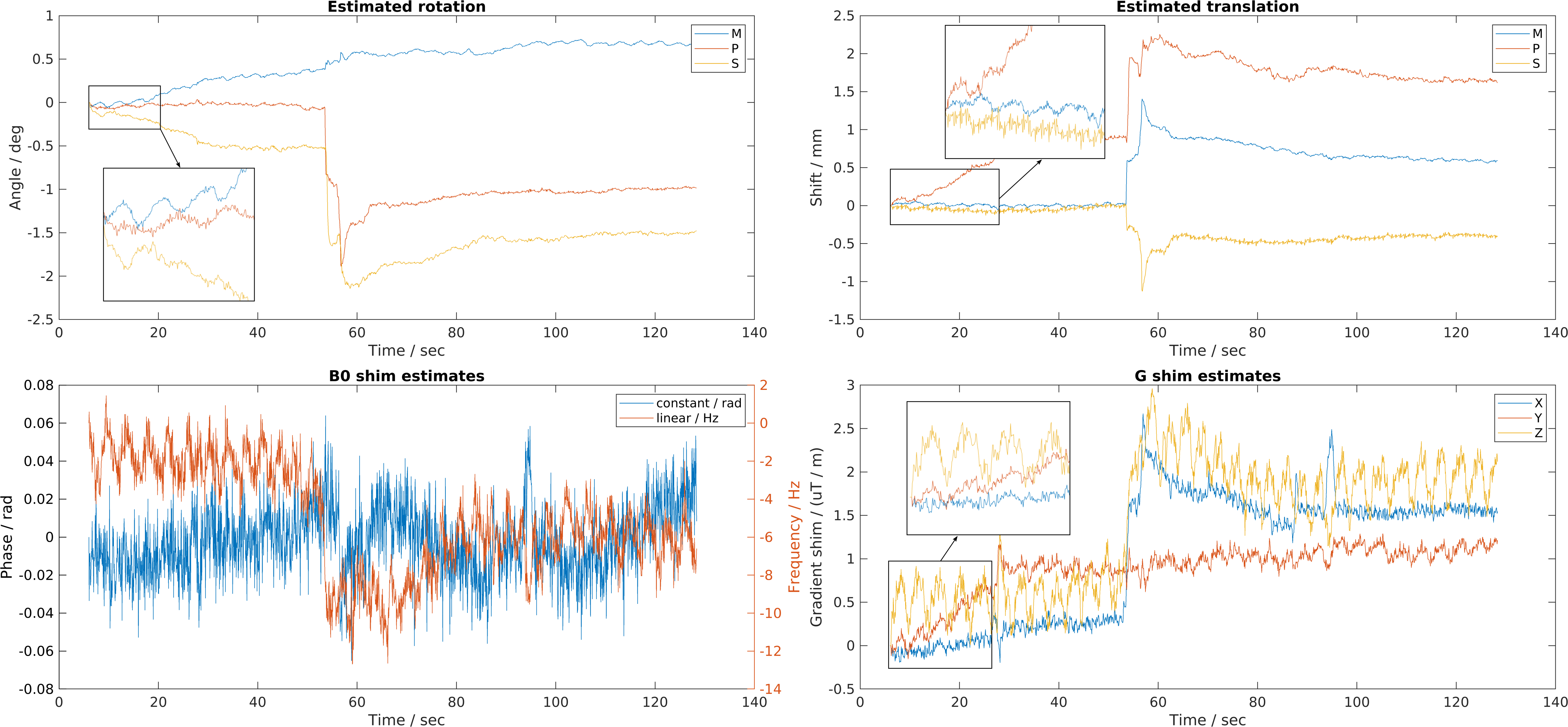
Figure 2 shows the imaging results of the experiments with geometry and shim perturbations. Both PMC methods perform well for rigid geometry perturbations, while ‘PMC + shim order 0’ shows strong ghosting due to the uncorrected gradient shim perturbations (green arrows). Figure 3 shows the motion and gradient shim parameters for the scan with shim perturbations (shown in Fig. 2B). In contrast to ‘PMC + shim order0’, the ‘PMC + shim order1’ with real-time 1st order shimming captures the shim perturbations, quickly reduces the bias on the other parameters and recovers the reference state.

Figure 4 compares in-vivo imaging results for instructed motion without PMC, with ‘PMC + shim order0’ and with ‘PMC + shim order1’. The latter gradient shim-calibrated method reduces the motion artifacts visibly. Figure 5 shows the estimated parameters for the ‘PMC + shim order1’ method. The motion and shim traces clearly show the instructed motion event as well as several physiological features, such as cardio-ballistic events in the S translations and Z shim variations at the breathing frequency.

Discussion and conclusion

The shim calibration exploits the sensitivity of navigators to field changes in the head frame and allows to correct for them up to first order in real-time. The method was shown to reduce field-induced biases on the other motion and field parameters and improves image quality in the phantom and in-vivo studies. To conclude, this study shows the feasibility of navigator-based motion and 1st order field correction with high precision and low sequence impact.

Acknowledgements

This work has received funding from the European Union’s Horizon 2020 research and innovation program under grant agreement No. 885876 (AROMA project).