Synopsis

Keywords: Machine Learning/Artificial Intelligence, Image Reconstruction

The application of generative models in MRI reconstruction is shifting researchers’ attention from the unrolled reconstruction networks to the probabilistically tractable iterations and permits an unsupervised fashion for medical image reconstruction.

Introduction

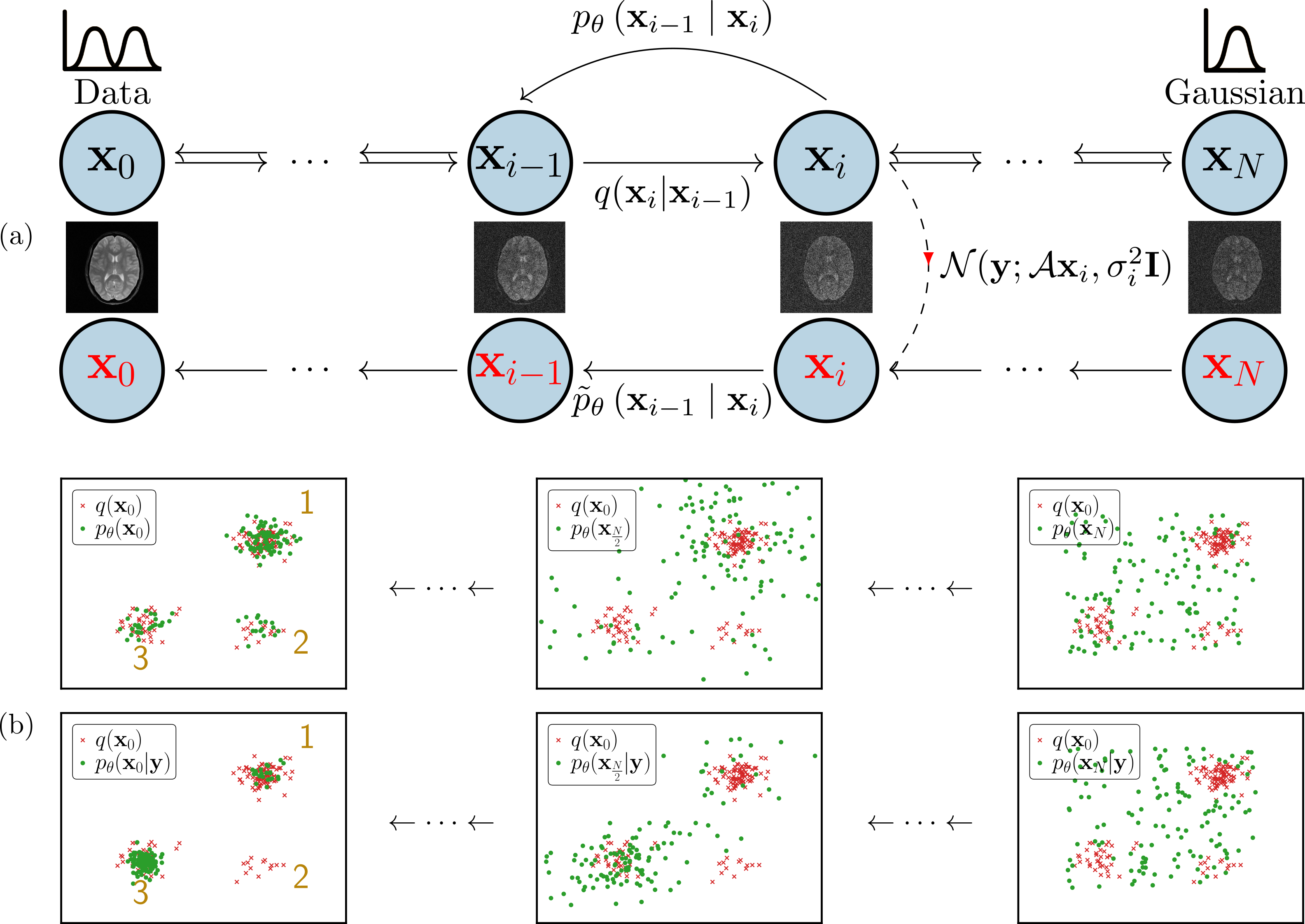
The application of generative models in MRI reconstruction is shifting researchers' attention from the unrolled reconstruction networks to the probablistically tractable iterations and permits an unsupervised fashion for medical image reconstruction [1-4].
We formulate the image reconstruction problem from the perspective of Bayesian inference, which enables efficient sampling from the learnt posterior probability distributions [1-2]. Different from conventional deep learning-based MRI reconstruction techniques, samples are drawn from the posterior distribution given the measured k-space using the Markov chain Monte Carlo (MCMC) method. The data-driven Markov chains are the reverse of a diffusion process that transfers the distribution of data to a known distribution (See Figure 1). Since the generative model learned from a image database is independent of the forward operator, this means the same pretrained models can be applied to k-space acquired with different sampling schemes or receive coils. Here, we present additional results in terms of the uncertainty of reconstruction, the transferability of learned information, and the comparison in the fastMRI challenge.

Theory

In order to compute the posterior probability $$$p(\mathbf{x}|\mathbf{y})$$$ for the image $$$\mathbf{x}$$$ given the measured k-space data $$$\mathbf{y}$$$, we need to modify the learned reverse process. We can achieve this by multiplying each of the intermediate distributions $$$p(\mathbf{x}_i)$$$ with the likelihood term $$$p(\mathbf{y}|\mathbf{x}_i)$$$ (see Figure 1). We use $$$\tilde{p}\left(\mathbf{x}_{i}\right)$$$ to denote the resulting sequence ofintermediate distributions\begin{equation} \tilde{p}\left(\mathbf{x}_{i}\right)\propto p\left(\mathbf{x}_{i}\right) p(\mathbf{y}|\mathbf{x}_i)\end{equation}up to the unknown normalization constant. Following [5], the transition from $$$\mathbf{x}_{i+1}$$$ to $$$\mathbf{x}_i$$$ of the modified reverse process is\begin{equation} \tilde{p}\left(\mathbf{x}_{i} \mid \mathbf{x}_{i+1}\right)\propto p\left(\mathbf{x}_{i} \mid \mathbf{x}_{i+1}\right) p(\mathbf{y}|\mathbf{x}_i). \end{equation} For the measument model of k-space, we express it as \begin{equation} p(\mathbf{y}|\mathbf{x}_i)=\mathcal{CN}(\mathbf{y};\mathcal{A}\mathbf{x}_i, \sigma_\eta^2\mathbf{I}).\end{equation}The sampling at each intermediate distribution of Markov transitions is performed with the unadjusted Langevin Monte Carlo [6] \begin{equation} \mathbf{x}_i^{k+1} \leftarrow \mathbf{x}_i^{k} + \frac{\gamma}{2}\nabla_{\mathbf{x}_i}\log \tilde{p}(\mathbf{x}_{i}^{k}\mid\mathbf{x}_{i+1}) + \sqrt{\gamma}\mathbf{z}, \label{eq:ld}\end{equation}where $$$\mathbf{z}$$$ is standard complex Gaussian noise $$$\mathcal{CN}(0, \mathbf{I})$$$. With the learned reverse process $$$p_{\boldsymbol{\theta}}\left(\mathbf{x}_i \mid \mathbf{x}_{i+1}\right)$$$, the log-derivative of $$$\tilde{p}_{\boldsymbol{\theta}}(\mathbf{x}_{i}\mid\mathbf{x}_{i+1})$$$ with respect to $$$\mathbf{x}_i$$$ is\begin{equation} \nabla_{\mathbf{x}_i}\log \tilde{p}_{\boldsymbol{\theta}}(\mathbf{x}_{i}\mid\mathbf{x}_{i+1}) = \nabla_{\mathbf{x}_i}\log p_{\boldsymbol{\theta}}\left(\mathbf{x}_i \mid \mathbf{x}_{i+1}\right) + \nabla_{\mathbf{x}_i}\log p(\mathbf{y}|\mathbf{x}_i),\end{equation}where\begin{equation} \nabla_{\mathbf{x}_i}\log p_{\boldsymbol{\theta}}\left(\mathbf{x}_i \mid \mathbf{x}_{i+1}\right) = \frac{1}{\tau_{i+1}^2}\left(\sigma_{i+1}^{2}-\sigma_{i}^{2}\right) \mathbf{s}_{\boldsymbol{\theta}}\left(\mathbf{x}_{i+1}, i\right)\end{equation}and \begin{align} \nabla_{\mathbf{x}_i}\log p(\mathbf{y}|\mathbf{x}_i) & = -\frac{1}{\sigma_\eta^2}(\mathcal{A}^{H} \mathcal{A}\mathbf{x}_i-\mathcal{A}^{H}\mathbf{y}_0).\end{align} For more details about how to learn reverse process and create measurement operator $$$\mathcal{A}$$$, please check our preprint [2].

Methods

In our preprint [2], we proposed Algorithm 1 for simulating samples from the posterior $$$p(\mathbf{x}|\mathbf{y})$$$ in which the score network [7] is used to construct Markov transition kernels. The following experiments are selected for this abstract. Codes and data to reproduce all experiments are made available in [8].

1. Multi-coil reconstruction
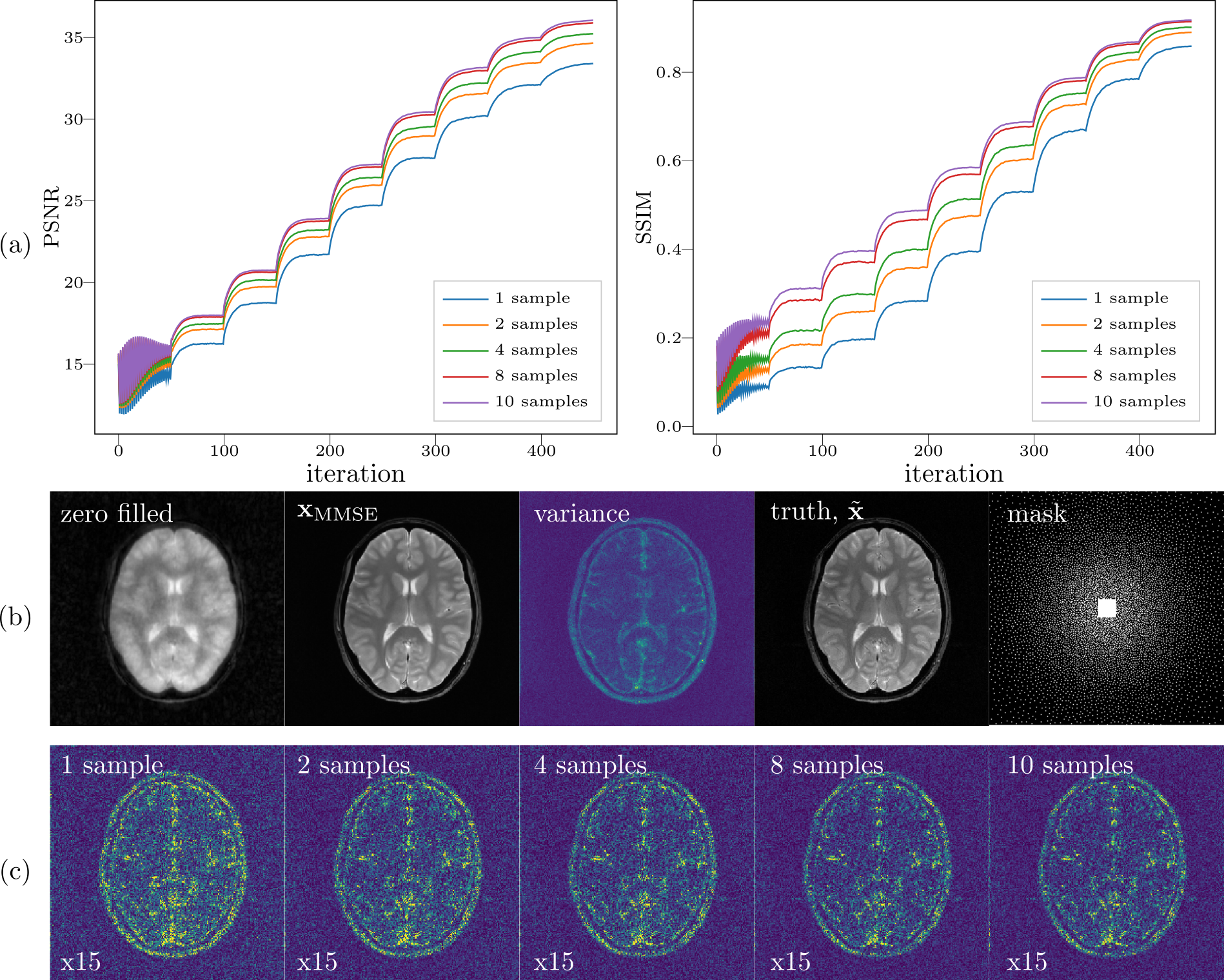
Multi-channel data points from k-space are randomly picked with variable density poisson-disc and the central 20$$$\times$$$20 region is fully acquired. The acquisition mask covers 11.8% k-space and the corresponding zero-filled reconstruction is shown Figure 2.We initialized 10 chains and the $$$\mathbf{x}_\mathrm{MMSE}$$$ was computed using different number of samples. The parameters in Algorithm 1 are $$$\mathrm{K}=50, \mathrm{N}=10, \lambda=13$$$.To visualize the process of sampling, we use peak-signal-noise-ratio (PSNR in dB) and similarity index (SSIM) as metrics to track intermediate samples.The comparisons are made between the magnitude of $$$\mathbf{x}_\mathrm{MMSE}$$$ and the ground truth $$$\tilde{\mathbf{x}}$$$ after normalized with $$$\ell_2$$$-norm.

2. Transferability
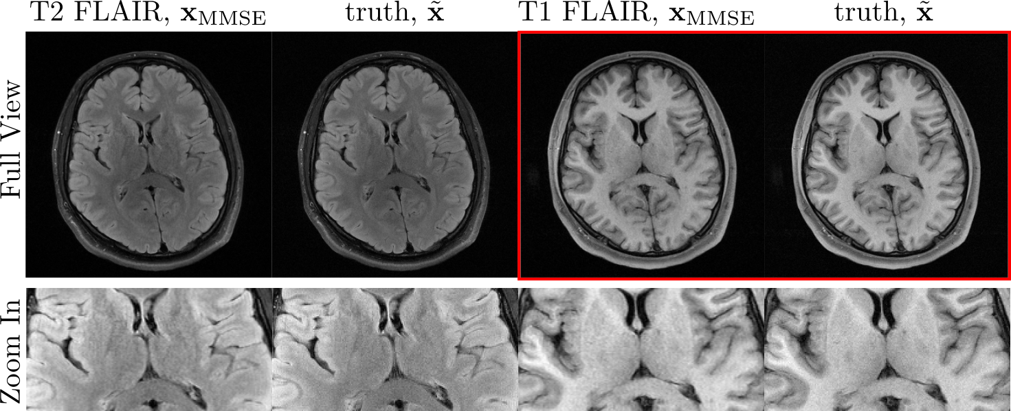
To investigate the transferability of learned prior information from T2 FLAIR images to other contrasts, we acquired T1-weighted (TR=2000ms, TI=900ms, TE=9ms) and T2-weighted (TR=9000ms, TI=2500ms, TE=81ms) FLAIR k-space data using a 2D multi-slice turbo spin-echo sequence with a 16-channel head coil at 3T (Siemens, 3T Skyra). The parameters in Algorithm 1 are $$$\mathrm{K}=2, \mathrm{N}=70, \lambda=20$$$.

3. Comparison to fastMRI challenge
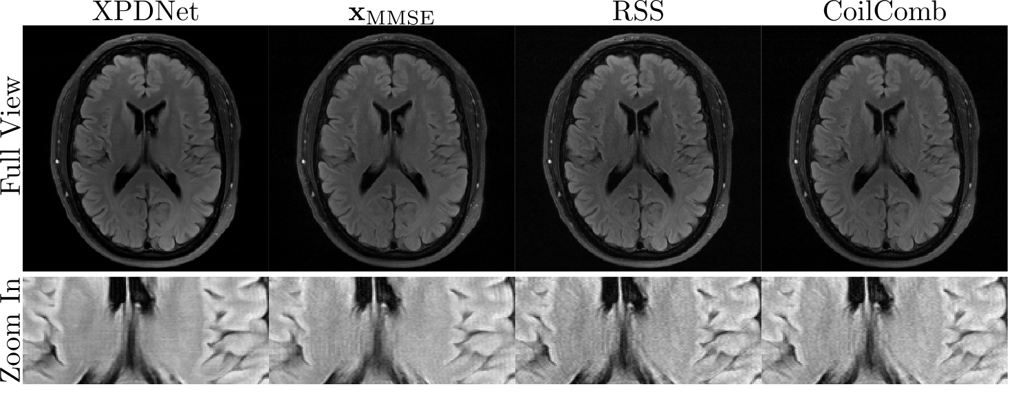
As a comparison to the unrolled neural network, the XPDNet is selected as the reference which ranked 2nd in the fastMRI challenge. Two networks were trained for acceleration factors 4 and 8, using retrospectively under-sampleddata from the fastMRI dataset [9] with equidistant Cartesian masks [10] and the trained models are available on [11]. For the proposed method, the parameters in Algorithm 1 are $$$K=4, N=90, \lambda=20$$$.

Results and Discussions

1. Multi-coil reconstruction
Comparing with the ground truth, the variance map mainly reflects the edge information, which can be interpreted by the uncertainty that is introduced by the undersampling pattern used in k-space where many high frequency data points are missing but the low frequency data points are fully acquired. In contrast to the single coil unfolding, the local spatial information from coil sensitivities reduces the uncertainties of missing k-space data. Moreover, error maps qualitatively correspond to the variance map, with larger errors in higher variance regions as shown in Figure 2.

2. Transferability
Figure 3 shows a score network trained with T2 FLAIR contrast used to reconstruct a T1 FLAIR image in comparison to a T2 FLAIR image. No loss can be observed.

3. Comparison to fastMRI challenge
As discussed in [12], the ground truth matters when computing metrics for the reconstruction. The RSS and Coil-combined are used as ground truth for XPDnet and $$$\mathbf{x}_\mathrm{MMSE}$$$.

Conclusion

The proposed reconstruction method combines concepts from machine learning, Bayesian inference and image reconstruction. In the setting of Bayesian inference, the image reconstruction is realized by drawing samples from the posterior term $$$p(\mathbf{x}|\mathbf{y})$$$ using data driven Markov chains, providing a minimum mean square reconstruction and uncertainty estimation. Furthermore, this method shows good performance in terms of transferabilities of contrasts and sampling patterns.

Acknowledgements

No acknowledgement found.