0985
Pharmacokinetic Parameters’ Distribution Estimation with Normalizing Flow in Dynamic Contrast-Enhanced Magnetic Resonance Imaging1College of Information Science and Electronic Engineering, Zhejiang University, Hangzhou, China, 2Key Laboratory of Biomedical Engineering of Ministry of Education, College of Biomedical Engineering and Instrument Science, Zhejiang University, Hangzhou, China, 3Department of Radiology, Qilu Hospital of Shandong University, Jinan, China, 4Department of Neurosurgery, Provincial Hospital Affiliated to Shandong First Medical University, Jinan, China, 5School of Medicine, Zhejiang University, Hangzhou, China
Synopsis
Keywords: Machine Learning/Artificial Intelligence, Data Analysis
The pharmacokinetic (PK) parameters extracted from the DCE-MRI provide valuable information but suffer from many sources of variability. Thus, the efficient and fast estimation of the distributions of these ambiguous PK parameters caused by variabilities could significantly improve the robustness and repeatability of DCE-MRI. The estimation of the PK parameters’ distributions provides a way to quantify the PK parameters’ values and variabilities simultaneously. In this study, we demonstrated the feasibility of the normalizing flow-based distribution estimation network (FPDEN) for PK parameters’ distribution estimation in DCE-MRI.
Introduction
The pharmacokinetic (PK) parameters extracted by the implementation of the dynamic contrast-enhanced magnetic resonance imaging (DCE-MRI) technique provide valuable information for clinical research and diagnosis. However, these PK parameters suffer from many sources of variability, e.g., signal-to-noise ratio (SNR)1, native T12, onset time3, arterial input function4 et al. Thus, the efficient and fast estimation of the distributions of these ambiguous PK parameters caused by variabilities could improve the robustness and repeatability of DCE-MRI.Maximum likelihood estimation (MLE)-based method can be utilized to solve for the mean and variance of these distributions. However, an appropriate posterior distribution is required, which is intractable, and the utilization of an inappropriate distribution assumption may degrade the PK parameters estimation performance5,6. In this work, the normalizing flow-based parameters distribution estimation network (FPDEN) was proposed to adaptively learn and estimate the posterior distribution of the PK parameters, thus further improving the accuracy of the parameter estimation.
Methods
The proposed FPDEN framework is shown in Fig.1 (a), which consists of a regression network for the estimation of the mean $$$\hat{\mathbf{\mu}}$$$ and uncertainty $$$\hat{\mathbf{\sigma}}$$$, as well as a normalizing flow model RealNVP7 to evaluate the shape of the parameter distribution.Normalizing flows learn to construct a complex distribution by transforming a simple distribution through an invertible mapping procedure. A potentially complex probability $$$x \sim p_X \in X$$$ can be calculated from a simple distribution $$$z=f(x) \sim p_z \in Z$$$ as: $$p_{X}(x) = p_{Z}(f(x))\left|\operatorname{det}\left(\frac{\partial f(x)}{\partial x^{T}}\right)\right|$$ where $$$\frac{\partial f(x)}{\partial x^{T}}$$$ represents the Jacobian of the invertible mapping . RealNVP is composed of a sequence of successive affine coupling layer (Fig. 1 (c)). Since the Jacobian in RealNVP is triangular, its determinant can be efficiently computed7. In this way, with a given arbitrary $$$x$$$ , the corresponding probability can be estimated through the above equation. With the reparameterization strategy8, the MLE loss can be written as: $$\begin{equation} \begin{split}\mathcal{L}_{mle}&=-\log p_{\theta,\phi}(\mathbf{x} \mid C_t') |_{\mathbf{x}=\mathbf{x_r}}\\&=-\log p_{\phi}(\overline{\mathbf{x}}_r)-\log \left|\operatorname{det} \frac{\partial \overline{\mathbf{x}}_r}{\partial \mathbf{x_r}}\right| \\ &=-\log p_{\phi}(\overline{\mathbf{x}}_r)+\log \hat{\mathbf{\sigma}}\end{split}\end{equation}$$ where $$${x_r}$$$ represents the label during train the model, $$$p_{\phi}(\overline{\mathbf{x}}_r)$$$ donates the learned zero-mean deformed distribution learned by the normalizing flow.
The DCE-MRI time-series signals were simulated by using the eTofts model9 to train and evaluate the proposed model. The contrast agent (CA) concentrations curves in the blood plasma $$$C_p$$$ used in this work were from 57 glioma patients’ DCE-MRI data. The proposed normalizing flow-based MLE loss $$$\mathcal{L}_{mle-flow}$$$ was compared with the conventional regression losses, i.e., $$$\mathcal{L}_{1}$$$ and $$$\mathcal{L}_{2}$$$ losses, and the one based on a multivariate Gaussian distribution10, i.e., the $$$\mathcal{L}_{mle-gau}$$$ loss, to examine how exactly the assumption of the posterior distribution affects the regression performance. The mean square error (MSE) and the signal reconstructed residual were calculated to evaluate the regression performance.
With Monte-Carlo simulation in World Health Organization (WHO) IV glioma tissues, the relationship between the uncertainty and the SNR, alone with the mean absolute error of the estimation, was analyzed to study the validity of uncertainty.
During the process of glioma grading, the PK parameters with large uncertainty were excluded, named uncertainty filtering (UF, Fig. 6 (a)). Thirty-three patients with pathologically confirmed high-grade gliomas (WHO grade III and grade IV) were enrolled in the Glioma grading task. The Receiver Operating Characteristic (ROC) and Area under Curve (AUC) were used to evaluate the classification performance.
Results
The regression models trained with maximum likelihood estimation loss outperformed those with the conventional losses (Fig. 2). Our method provided better parameter estimation accuracy than the other methods (including the Gaussian distribution hypothesis) alone with lower signal fitting residuals.As can be observed from Fig.3 (a)-(c), as the SNR is decreased, the uncertainty of all the three parameters $$$K^{\mathrm{trans}}$$$, $$$V_{p}$$$, and $$$V_{e}$$$ becomes bigger. Meanwhile, there is a strong correlation, especially for $$$K^{\mathrm{trans}}(R^2=0.982)$$$ and $$$V_{e}(R^2=0.977)$$$, between the uncertainty and the standard deviation (SD) of the estimated value.
UF can improve the classification performance of glioma grading. Fig. 4 (b) demonstrates that the use of $$$V_{e}$$$ for glioma grading is effective ($$$AUC>0.5$$$) only after UF is used and UF can increase the AUC of logistic regression from 0.639 to 0.657.
Discussion
Figs.5 (a)-(c) depict the correlation between each pair of parameters from the learned zero-mean deformed PK parameters distribution. The marginal distributions of the target parameters and the top 5 best-fitted distributions are also given in Figs.5 (d)-(f). Bias still exists between the best-fitted distribution and the targeted distribution, suggesting that the presumption of a posterior distribution of the PK parameters inevitably introduces empirical errors.The estimated standard deviation overestimates the standard deviation of the PK parameter values obtained from the regression network output $$$\hat{\mathbf{\mu}}$$$ in the Monte-Carlo simulations. The uncertainty $$$\hat{\mathbf{\sigma}}$$$ estimated for each PK parameter can be defined as the standard deviation of the marginal distribution of the parameter and should be treated as the network estimation error. The lower variance proves the stability of the regression model.
Conclusion
The proposed FPDEN can be used to automatically learn the posterior distribution of the PK model parameters, thus effectively improving the accuracy of the parameter estimation process. The uncertainty provided by the framework can also boost the performance of downstream tasks that depend on the PK parameters.Acknowledgements
This work was supported in part by the National NaturalScience Foundation of China (NSFC) under Grant 82172050, Grant81873894, Grant 82111530201, and Grant 82222032; in part by theNatural Science Foundation of Zhejiang Province, China, under GrantLR20H180001; in part by the MOE Frontier Science Center for BrainScience & Brain-Machine Integration, Zhejiang University.References
1. Yuan J, Chow SKK, Yeung DKW, Ahuja AT, King AD. Quantitative evaluation of dual-flip-angle T 1 mapping on DCE-MRI kinetic parameter estimation in head and neck. Quantitative Imaging in Medicine and Surgery. 2012;2(4). https://qims.amegroups.com/article/view/1309
2. Heye T, Boll DT, Reiner CS, Bashir MR, Dale BM, Merkle EM. Impact of precontrast T10 relaxation times on dynamic contrast-enhanced MRI pharmacokinetic parameters: T10 mapping versus a fixed T10 reference value. Journal of Magnetic Resonance Imaging. 2014;39(5):1136-1145. doi:10.1002/jmri.24262
3. Orton MR, Collins DJ, Walker-Samuel S, et al. Bayesian estimation of pharmacokinetic parameters for DCE-MRI with a robust treatment of enhancement onset time. Phys Med Biol. 2007;52(9):2393-2408. doi:10.1088/0031-9155/52/9/005
4. Dikaios N, Atkinson D, Tudisca C, et al. A comparison of Bayesian and non-linear regression methods for robust estimation of pharmacokinetics in DCE-MRI and how it affects cancer diagnosis. Computerized Medical Imaging and Graphics. 2017;56:1-10. doi:10.1016/j.compmedimag.2017.01.003
5. Kelm BM, Menze BH, Nix O, Zechmann CM, Hamprecht FA. Estimating Kinetic Parameter Maps From Dynamic Contrast-Enhanced MRI Using Spatial Prior Knowledge. IEEE Transactions on Medical Imaging. 2009;28(10):1534-1547. doi:10.1109/TMI.2009.2019957
6. Bliesener Y, Acharya J, Nayak KS. Efficient DCE-MRI Parameter and Uncertainty Estimation Using a Neural Network. IEEE Trans Med Imaging. 2020;39(5):1712-1723. doi:10.1109/TMI.2019.2953901
7. Dinh L, Sohl-Dickstein J, Bengio S. Density estimation using Real NVP. arXiv:160508803 [cs, stat]. Published online February 27, 2017. Accessed December 12, 2021. http://arxiv.org/abs/1605.08803
8. Li J, Bian S, Zeng A, et al. Human Pose Regression with Residual Log-likelihood Estimation. arXiv:210711291 [cs]. Published online July 31, 2021. Accessed September 5, 2021. http://arxiv.org/abs/2107.11291
9. Tofts PS. T1-weighted DCE Imaging Concepts: Modelling, Acquisition and Analysis. 26:31-39.
10. Do CB. The multivariate gaussian distribution. Section Notes, Lecture on Machine Learning, CS. 2008;229.
Figures
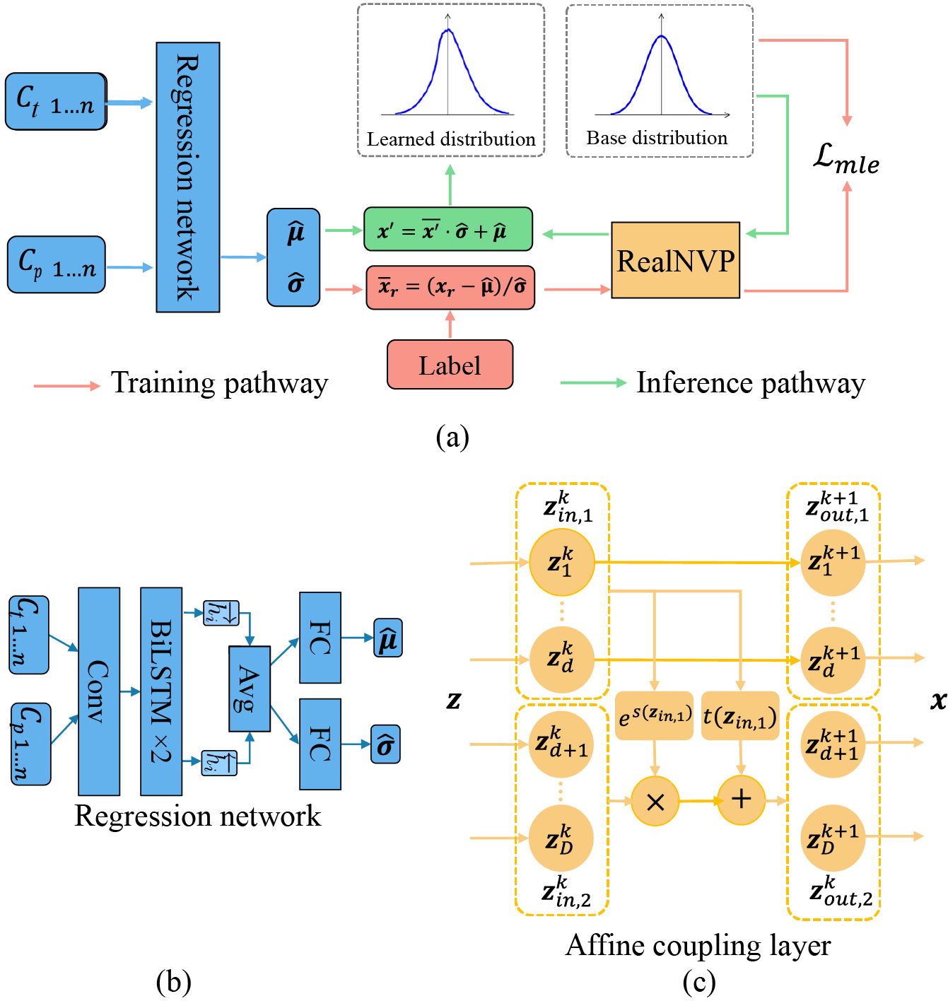
Fig. 1. Schematic illustration of the proposed framework and network architecture. In (a), the regression network used the CA concentration in the tissue $$$C_t$$$ and CA concentration $$$C_p$$$ in the blood plasma as inputs to estimate the mean and variance of the PK parameters. Reparameterization techniques were applied to calculate the likelihood of the output. (b) depicts the architecture of the LSTM-based regression network. The normalizing flow model RealNVP in (a) consists of a sequence of affine coupling layers, and an affine coupling layer is provided in (c).
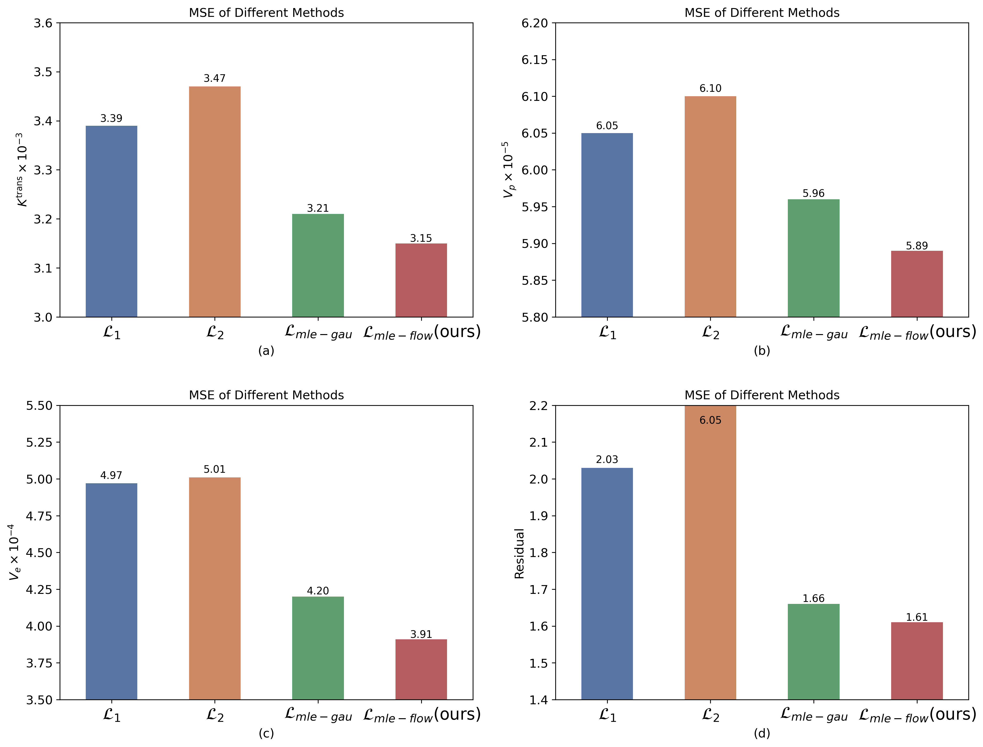
Fig. 2. The quantitative comparison of the regression model results trained with different losses on the test dataset.
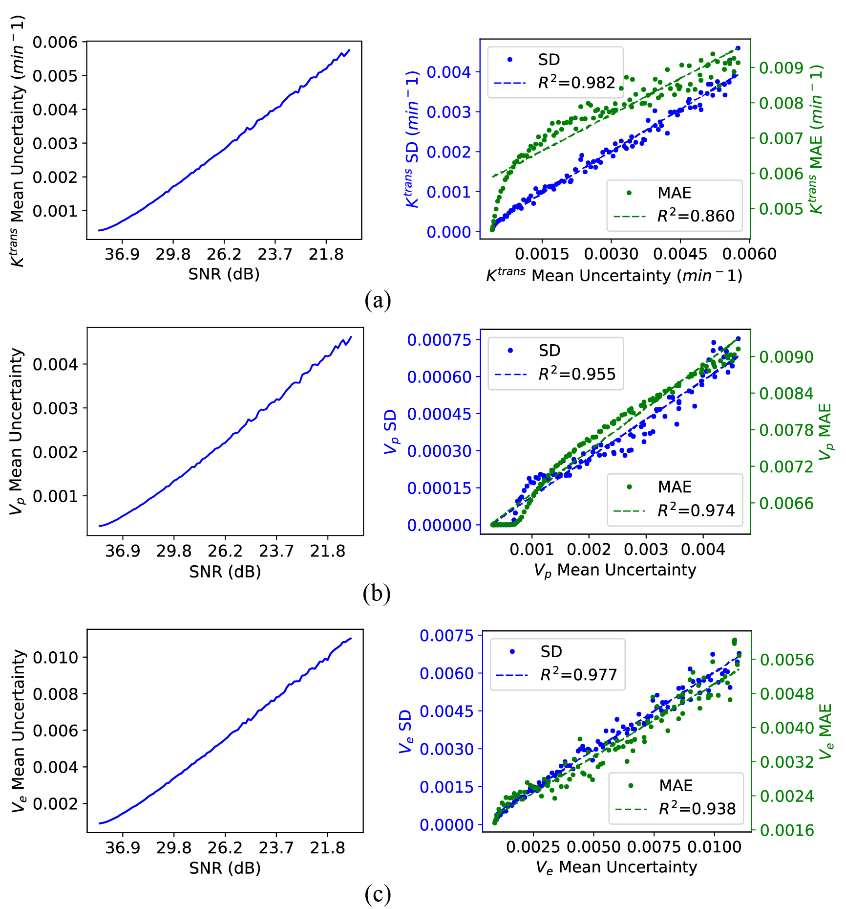
Fig. 3. Depiction of the mean uncertainty, estimation MAE, and estimation SD for the different noise levels. Here a DCE-MRI signal mimicking WHO IV glioma tissue was simulated, and 100 noise realizations were performed for each SNR. The left column of (a) - (c) shows the relationship between the certainty and the SNR. In the right column, the blue dots represent the inferences SD and the green dots stand for the inferences MAE in each case of uncertainty (each uncertainty comes from a particular SNR). The coefficient of Determination ($$$R^2$$$) is marked in the legend.
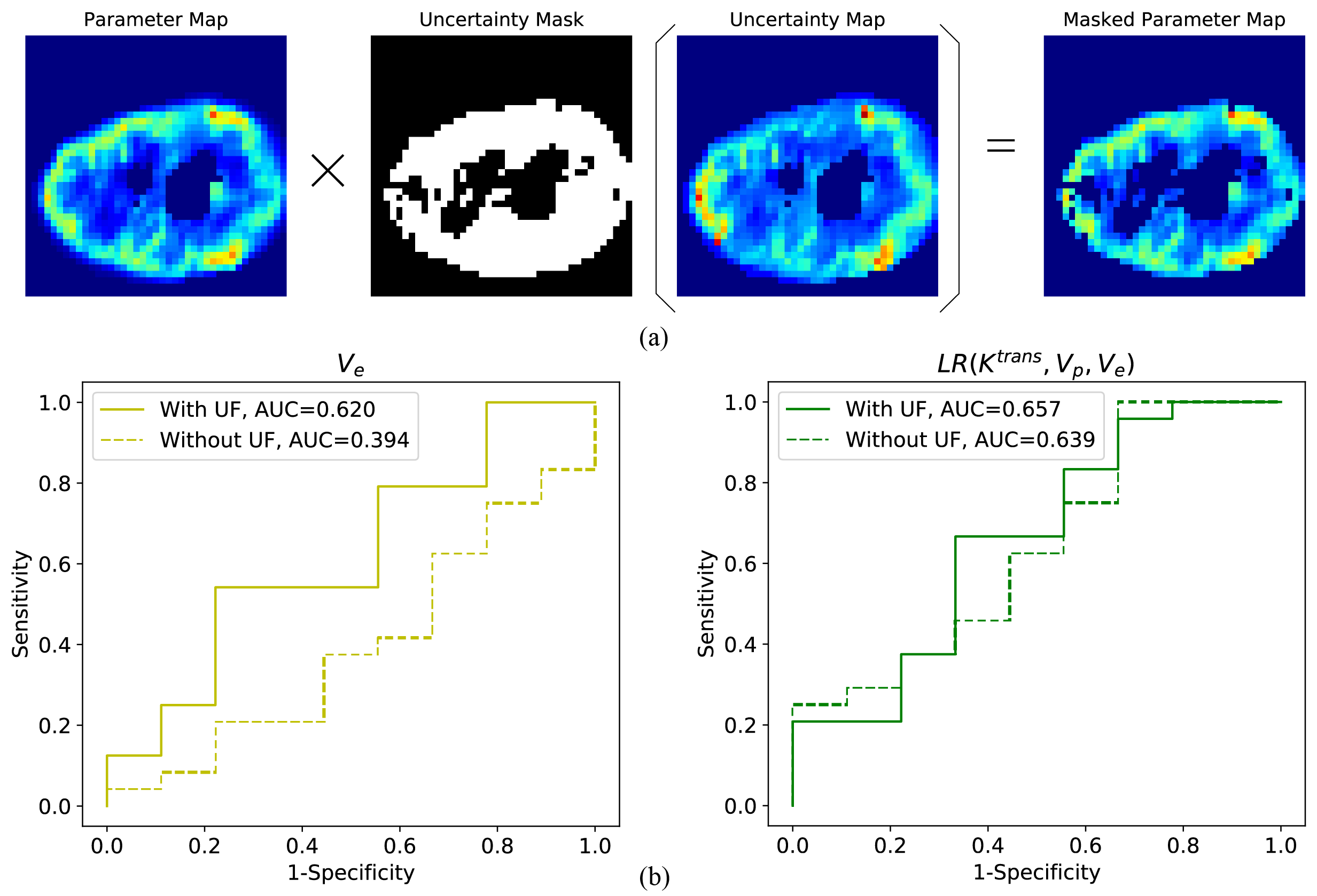
Fig. 4. Filtering out of voxels with large parametric uncertainty can improve the WHO grading between III and IV of gliomas. The uncertainty maps were used to generate an uncertainty mask according to the UF thresholds to filter out unreliable parameters so that only reliable parameters were used to calculate parameter averages within the tumor regions. The data processing process is shown in (a). Grade IV is defined as a positive sample and (b) presents the ROC curves for glioma classification using $$$V_e$$$ and logistic regression. The AUCs are written in the legends.
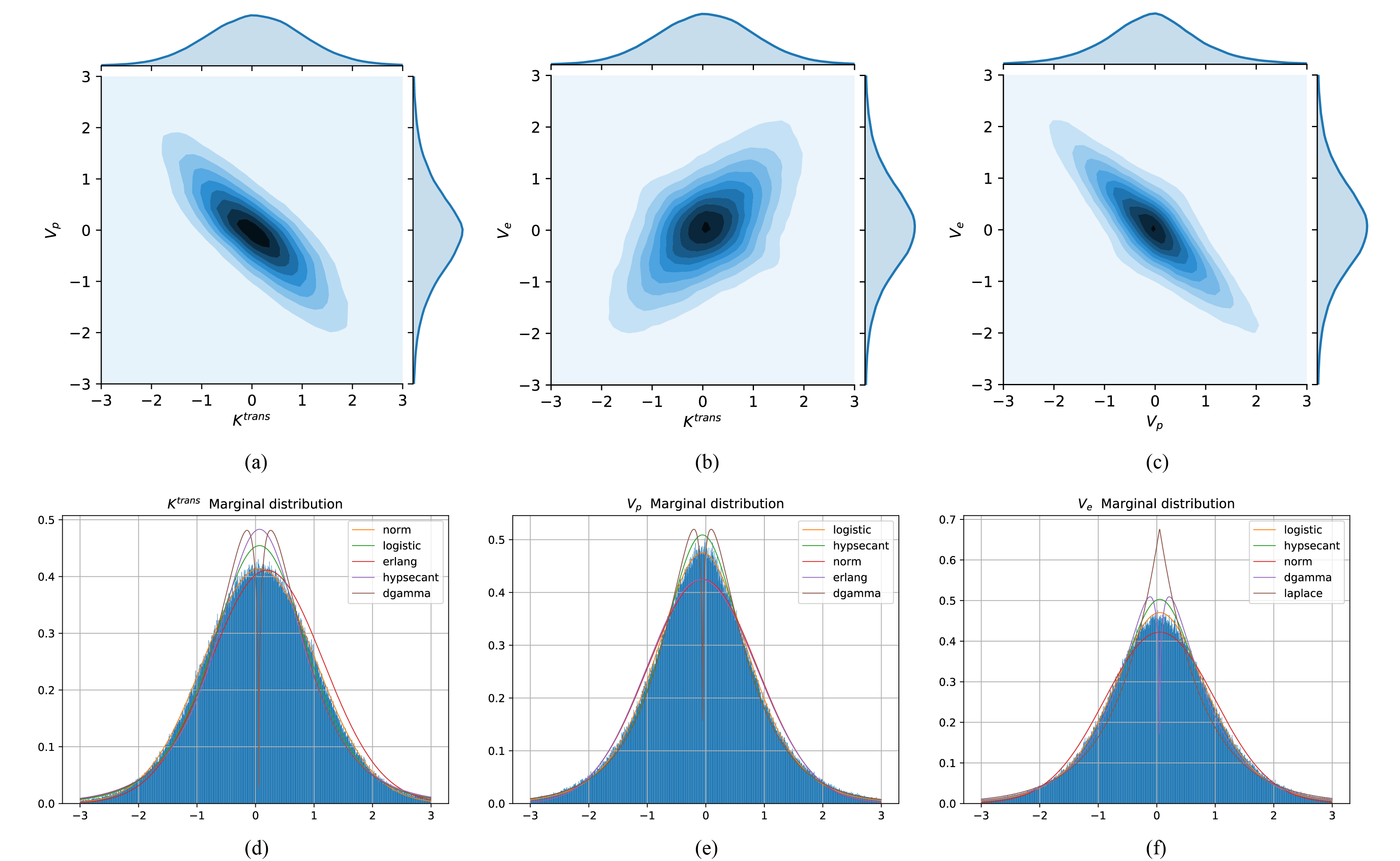
Fig. 5. The joint distribution between every two parameters and the parameter marginal distribution of PK parameters of eTofts learned by the proposed normalizing flow model. The contour maps of the probability density in the two-dimensional space are shown in (a) - (c), respectively. Figs. (d) - (f) correspond to the marginal distribution of $$$K^{\mathrm{trans}}$$$, $$$V_{p}$$$, and $$$V_{e}$$$, respectively. Common distributions were used to fit these distributions as best as possible. These distribution fitting curves were sorted based on the sum of square Error.