Synopsis

Keywords: Diffusion/other diffusion imaging techniques, Data Acquisition

In brain dMRI, microstructure parameters of fiber fascicles, such as compartment fractions, exchange, diffusivities, relaxation rates, and structural disorder, are highly sought after. They can be accessed by sampling multiple diffusion weightings, b-tensor shapes, diffusion and/or echo times. Yet most scan time is spent oversampling the fiber orientation distribution function – because factoring it out nominally requires rotational invariants like the spherical mean. We show how to measure multiple inequivalent combinations of $$$(b,\,\Delta)$$$, while spending single gradient directions per unique combination. We recover signal’s rotational invariants for each one and use them for biophysical modeling of white and gray matter.

Introduction

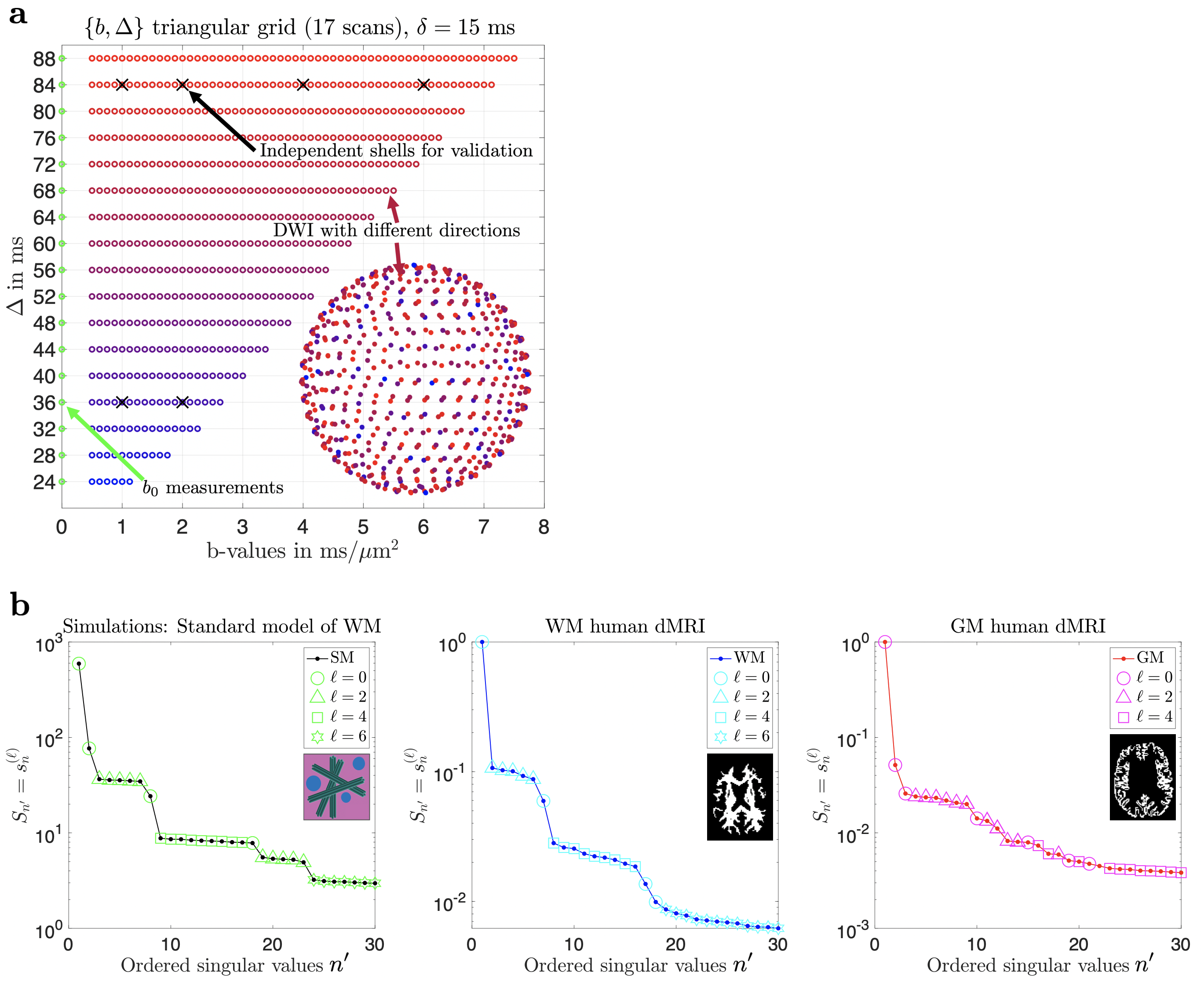
Using brain diffusion MRI (dMRI), we often aim to extract microstructure parameters of fiber fascicles (such as compartment fractions, diffusivities, relaxation rates, exchange between compartments, and structural disorder)^1-6. These can be revealed by sampling different diffusion weightings, tensor shapes, diffusion and echo times. Yet most of our scan time is typically spent on oversampling the fiber orientation distribution function (fODF) – simply because factoring out the fODF nominally requires constructing spherical means^7-8, or higher-order rotational invariants^9,10.
Here we show how to measure multiple combinations of experimental parameters – e.g. distinct combinations of diffusion weighting $$$b$$$ and diffusion time $$$\Delta$$$ – while spending only a single gradient direction $$$\hat{\mathbf{g}}$$$ per unique combination $$$(b,\,\Delta)$$$. In this way, we measure 550 distinct combinations of $$$(b,\,\Delta)$$$ in under one hour and recover their signal rotational invariants, which would have taken 30 hours if acquired instead for shells with 30 directions each. Finally, we apply our methods in vivo to observe the functional forms of fiber fascicles in both human white and gray matter, study diffusion time dependence, and use this data to estimate white and gray matter biophysical models.

Theory

The idea is to relate the singular value decomposition (SVD) of the signal from many voxels to the SVD of the (unknown) fiber fascicle response kernel, achieved using factorization in spherical harmonics (SH) space.
SH Factorization: The voxelwise diffusion signal of many tissues, e.g. white and gray matter, can be modeled as a convolution over the sphere^1,11-13:
$$S\left(b,\Delta,\hat{\mathbf{g}}\mid\!\,x,p_{\ell\,\!m}\right)=\int_{\mathbb{S}^{2}}d\hat{\mathbf{n}}\,\mathcal{K}(b,\Delta,\hat{\mathbf{g}}\cdot\hat{\mathbf{n}}\mid\,\!x)\,\mathcal{P}(\hat{\mathbf{n}}\mid\!\,p_{\ell\,\!m}),\quad(1)$$
where $$$b,\,\Delta,$$$ and $$$\hat{\mathbf{g}}$$$ define the measurement, $$$x=[f_a,D_a,T_{2,a},...,\tau_\mathrm{ex},...]$$$ contains the parameters describing the fiber response $$$\mathcal{K}$$$ (kernel), and $$$\mathcal{P}(\hat{\mathbf{n}}\mid\,\!p_{\ell\,\!m})=\sum_{\ell\,\!m}p_{\ell\,\!m}\,Y_{\ell\,\!m}(\hat{\mathbf{n}})$$$ is the fODF, represented by its spherical harmonics coefficients $$$p_{\ell\,\!m}$$$. Any spherical convolution can be replaced by a product in the SH basis:
$$S\left(b,\Delta,\hat{\mathbf{g}}\mid\,\!x,p_{\ell\,\!m}\right)=\sum_{\ell\,\!m}S_{\ell\,\!m}(b,\Delta)\,Y_{\ell\,\!m}(\hat{\mathbf{g}})=\sum_{\ell\,\!m}\mathcal{K}_{\ell}(b,\Delta\mid\!\,x)\,p_{\ell\,\!m}\,Y_{\ell\,\!m}(\hat{\mathbf{g}}).\quad(2)$$
where $$$\mathcal{K}_{\ell}$$$ are the kernel's rotational invariants.
SVD of kernel $$$\mapsto$$$ SVD of signal: While $$$\mathcal{K}_{\ell}$$$ are generally unknown, they admit the SVD factorization into protocol- and tissue-dependent components $$$u_n^{(\ell)}$$$ and $$$v_n^{(\ell)}$$$:
$$\mathcal{K}_\ell(b,\Delta\mid\,\!x)\simeq\sum_{n=1}^{N_{\ell}}s_{n}^{(\ell)}\,u_{n}^{(\ell)}(b,\Delta)\,v_{n}^{(\ell)}(x).\quad(3)$$
If we were to determine the components of Eq. (3) from a measurement, we could reconstruct the kernel $$$\mathcal{K}_{\ell}$$$. The way to measure $$$u_n^{(\ell)}$$$ and $$$v_n^{(\ell)}$$$ is to realize that, if we substitute Eq. (3) into Eq. (2), the signal
$$S\left(b,\Delta,\hat{\mathbf{g}}\mid\,\!x,p_{\ell\,\!m}\right)\simeq\sum_{n\ell\,\!m}s_{n}^{(\ell)}\,u_{n}^{(\ell)}(b,\Delta)\,Y_{\ell\,\!m}\left(\hat{\mathbf{g}}\right)\,v_{n}^{(\ell)}(x)\,p_{\ell\,\!m},\quad(4)$$
acquires an SVD form
$$S\left(b,\Delta,\hat{\mathbf{g}}\mid\!\,x,p_{\ell\,\!m}\right)\simeq\sum_{n^{\prime}}^NS_{n^{\prime}}\,U_{n^{\prime}}(b,\Delta,\hat{\mathbf{g}})\,V_{n^{\prime}}\left(x,p_{\ell\!\,m}\right),\quad(5)$$
where S is the diagonal matrix of singular values, and U and V depend solely on acquisition parameters and tissue, respectively. To ensure that $$$S_{n'}$$$ decay fast with $$$n'$$$, the signal SVD should be performed across voxels of the same tissue type, probing the same kernel across the range of values of its parameters $$$x$$$ and fODF components $$$p_{\ell\,\!m}$$$.
We now relate the components of Eq. (5) to those of Eq. (4) by assigning ``quantum numbers" $$$n,\,\ell,\,m$$$ to the columns of U, i.e. mapping $$$n'\rightarrow\{n,\ell,m\}$$$. This is done by projecting U on $$$Y_{\ell\,\!m}\left(\hat{\mathbf{g}}\right)$$$ and applying Wigner D-matrices to ``rotate'' U to the conventional SH basis. This results in the ``multiplets" (see Fig. 1b) with singular values $$$s_n^{(\ell)}$$$, ($$$2\ell+1$$$)-degenerate with respect to $$$m$$$, akin to atomic orbitals in the periodic table. We can then define protocol and tissue basis functions:
$$\alpha_{n\ell\,\!m}=u_{n}^{(\ell)}(b,\Delta)\,Y_{\ell\,\!m}\left(\hat{\mathbf{g}}\right),\quad\gamma_{n\ell\,\!m}=v_{n}^{(\ell)}(x)\,p_{\ell\,\!m},\quad(6)$$
where the $$$L_2$$$ norm over each ``multiplet" combined with sign estimation provides
$$\begin{aligned} \alpha_{n\ell}&=||\alpha_{n\ell\,\!m}||^{(m)}=\sqrt{\sum_{m}\alpha_{n\ell\,\!m}^{2}}=\sqrt{\tfrac{2\ell+1}{4\pi}}\,|u_{n}^{(\ell)}(b,\Delta)|,&&\tilde{\alpha}_{n\ell}=\alpha_{n\ell}\times\mathrm{sign}(u_{n}^{(\ell)}(b,\Delta)),\\\,\!\gamma_{n\ell}&=||\gamma_{n\ell\,\!m}||^{(m)}=\sqrt{\sum_{m}\gamma_{n\ell\,\!m}^{2}}=\sqrt{4\pi(2\ell+1)}\,p_{\ell}\,|v_{n}^{(\ell)}(x)|,&&\tilde{\gamma}_{n\ell}=\gamma_{n\ell}\times\mathrm{sign}(v_{n}^{(\ell)}(x)).\end{aligned}\quad(7)$$
These can be combined to recover the signal rotational invariants without knowing the kernel's functional form:
$$S_\ell\left(b,\Delta\mid\,\!x,p_{\ell}\right)=p_\ell\,\mathcal{K}_\ell(b,\Delta\mid\,\!x)=\tfrac{1}{2\ell+1}\,\sum_{n}\tilde{\alpha}_{n\ell}\,\tilde{\gamma}_{n\ell}.\quad(8)$$

Experiments

A 25-year-old male volunteer underwent 3T MRI (Siemens Magnetom Prisma) using a 32-channel head coil. A monopolar PGSE (Siemens WIP-511E) diffusion weighting sequence was used to acquire 550 diffusion-weighted images (DWIs) distributed into unique $$$(b,\,\Delta)$$$ pairs: $$$b\in[0,7.5]\,\mathrm{ms/\mu\,\!m^2},\,\Delta\in[24,88]\,\mathrm{ms}$$$, sampled in a triangular grid (see Fig. 1a), $$$\delta=15\,\mathrm{ms},\,t_\mathrm{acq}=55\,\mathrm{min}$$$. The 550 directions were uniformly distributed in the sphere and randomly assigned to each $$$(b,\,\Delta)$$$. For validation purposes, 6 complete shells were acquired at $$$(b\,[\mathrm{ms/\mu\,\!m^2}],\,\Delta\,[\mathrm{ms}],\,\mathrm{N}_\mathrm{dirs})=\{(1,36,24);(2,36,48);(1,84,24);(2,84,48);(4,84,48);(6,84,60)\},\,t_\mathrm{acq}=25\,\mathrm{min}$$$. Imaging parameters: voxel size$$$\,=2\times2\times2\,$$$mm$$$^3,\,\mathrm{TE}=120\,\mathrm{ms},\,\mathrm{TR}=5\,\mathrm{s},\,\mathrm{bandwidth}=2275\,\mathrm{Hz/Px},\,R_\mathrm{GRAPPA}=2,\,\text{partial Fourier}=6/8,\,\mathrm{Multiband}=2$$$.

Results

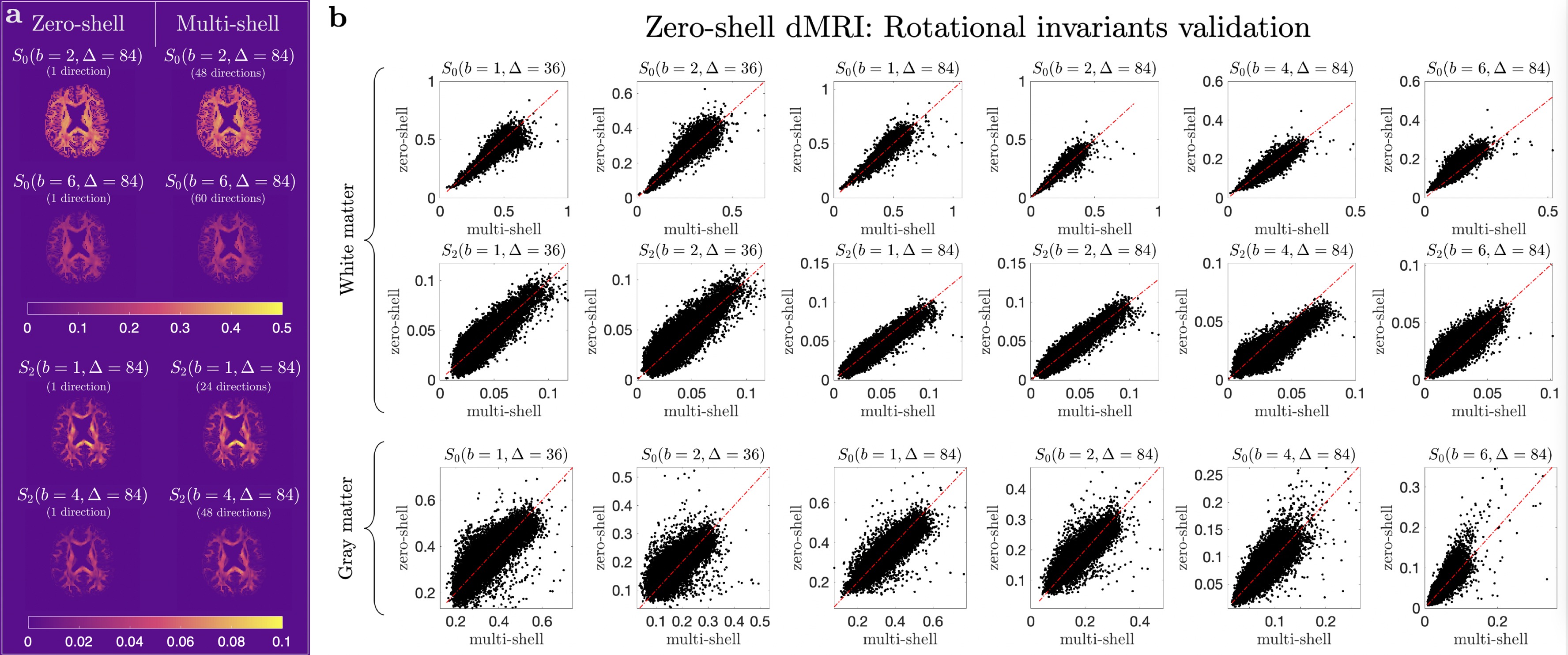
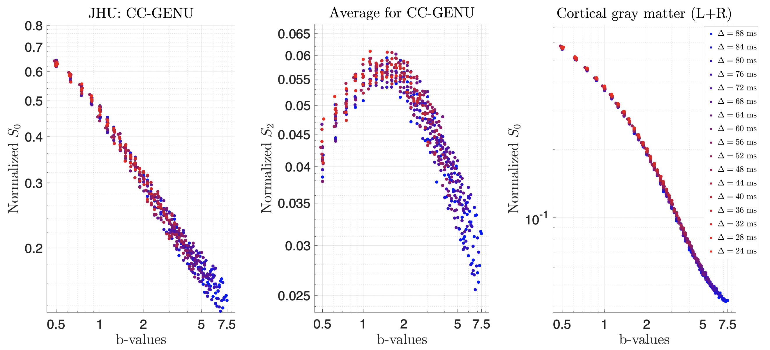
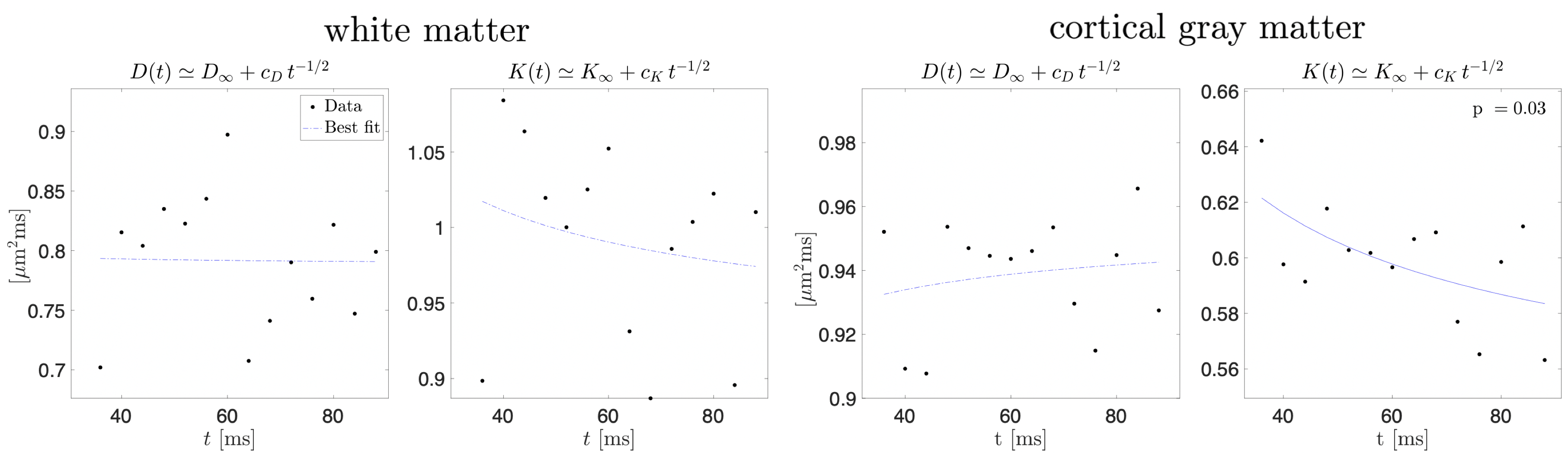
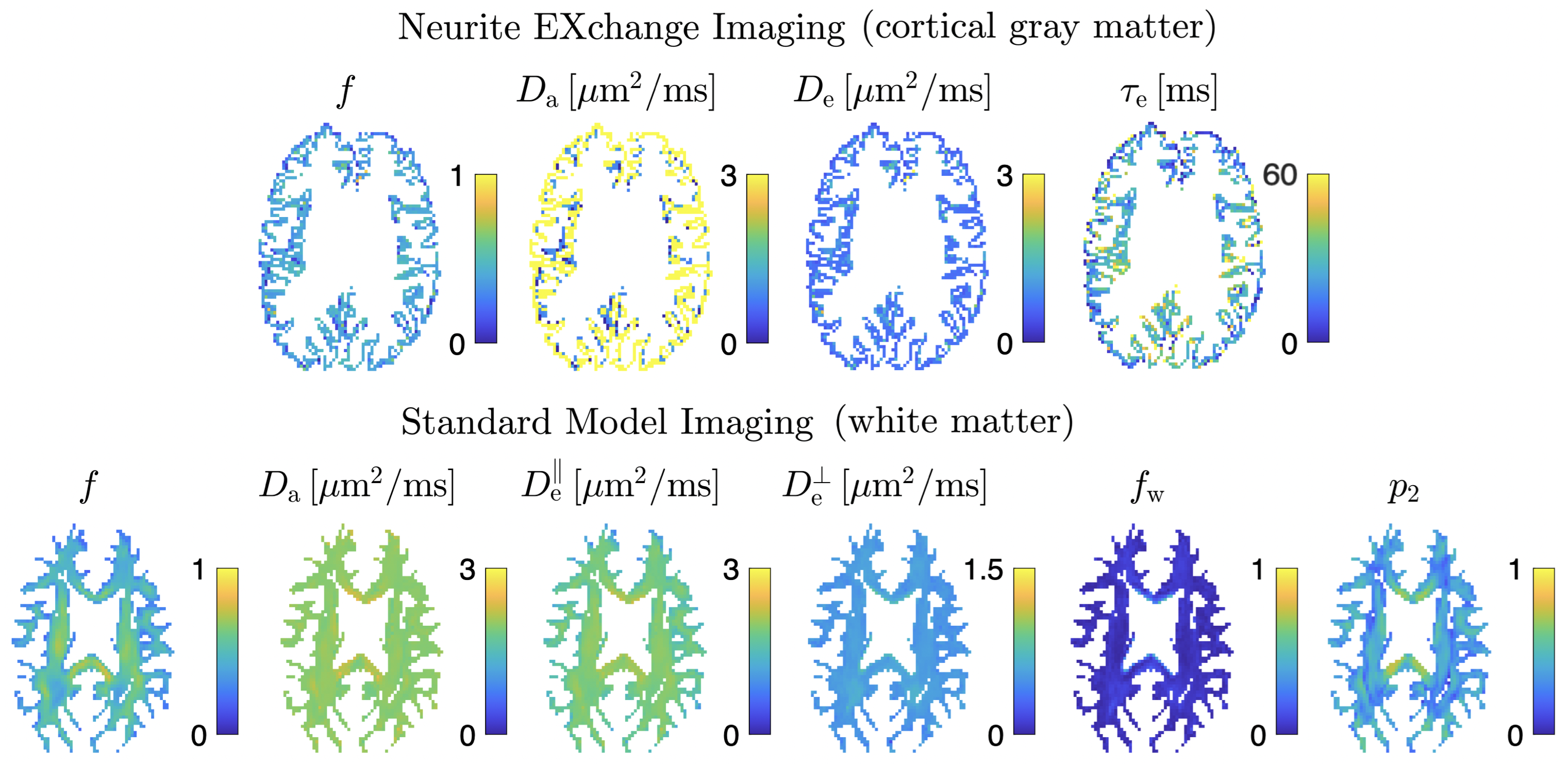
SVD of simulated voxels according to the Standard Model of diffusion in white matter, as well as measured human WM and GM, are shown in Fig. 1b. The presence of the multiplets of exactly $$$2\ell+1$$$ elements in the data supports the assumption of a convolution in the selected group of voxels. Furthermore, rotational invariants maps reconstructed using Eq. (8) for different WM/GM regions are shown in Fig. 2a, together with scatter plots showing high agreement with the validation shells. Their dependence on $$$b$$$ for WM/GM regions is shown in Fig. 3. We can use rotational invariants to compute DTI/DKI and study their time dependence (Fig. 4, in agreement with¹⁴), or to estimate any biophysical models like the Standard Model¹⁵ in WM or Neurite Exchange Imaging¹² for GM (Fig. 5).

Discussion and Conclusion

We measured in vivo brain dMRI signal rotational invariants in 550 unique $$$(b,\,\Delta)$$$ combinations without sampling complete shells on each of them. Our framework is built upon the convolution of the kernel and fODF but no assumptions are made about the functional form of the tissue response function which is allowed to vary between voxels. This method, readily extendable for B-tensor shapes, TE, etc, provides massive time savings for techniques requiring dense sampling of the multi-dimensional MRI acquisition space^15-19. The number of distinct $$$s_n^{(\ell)}$$$ above the noise floor provides an upper limit to the number of degrees of freedom needed to model the kernel.

Acknowledgements

This work has been supported by NIH under NINDS award R01 NS088040 and NIBIB awards R01 EB027075 and P41 EB017183. The authors are grateful to Sune N. Jespersen for fruitful discussions and to Thorsten Feiweier for providing the WIP-511E sequence.