Synopsis

Keywords: RF Pulse Design & Fields, High-Field MRI

A fast B₁⁺ mapping sequence such as saturation-prepared turbo FLASH (satTFL) is desirable for online pulse design at ultra-high field, but it often results in inaccuracies. Previous work performed linear fitting of the B₁⁺ magnitude obtained with the satTFL over that of the longer but more accurate Actual Flip angle Imaging (AFI) sequence to obtain calibration parameters that would correct the satTFL B₁⁺ on the fly for brain imaging. In this work we introduce a new machine-learning-based method that uses additional features to create a more precise and less location-dependent accuracy.

Introduction

Ultra-high field MRI, along with radiofrequency (RF) parallel transmission, offer opportunities in terms of signal-to-noise ratio and flexibility, but at the expense of challenges for calibration and calibration time¹. Methods relying on parallel transmission generally necessitate the acquisition of $$$B_1^+$$$ field maps.

The saturation-prepared turbo FLASH method² (satTFL) is fast – it can map the $$$B_1^+$$$ field in about 30s for an 8-transmit-channel system – which makes it well suited for online pulse design. However, as shown in previous studies^3,4, it lacks the accuracy needed for some design techniques. Sedlacik et al.³ have presented a way to calibrate the satTFL against the more accurate but slower Actual Flip angle Imaging (AFI) mapping sequence⁵, in the brain, by acquiring both maps on a set of subjects and performing a linear fitting of the $$$B_1^+$$$ magnitude of paired voxels. However, the quality of the correction was spatially dependent.

The present work investigates the use of supervised machine learning to correct for spatially dependant inaccuracies of the satTFL $$$B_1^+$$$ map.

Methods

26 healthy volunteers underwent a scan on a 7T scanner (MAGNETOM Terra, Siemens Healthcare, Erlangen, Germany) using an 8Tx/32Rx-channel head coil (Nova Medical, Wilmington, MA, USA). Human subject scanning was approved by the Institutional Research Ethics Committee (HR-18/19-8700).

Two sets of brain $$$B_1^+$$$ maps were acquired on each subject with channels combined in circular polarisation (CP), with matched imaging positions, fields of view (FOV) and resolutions. The sat-TFL was acquired with the same protocol as the vendor-provided automatic measurement: 25 slices of thickness 5mm and 5mm spacing, in-plane FOV: 256x256mm², matrix: 64x64, nominal flip angle (FA): $$$\alpha_\mathrm{nom,satTFL}=90^\circ$$$, scan time: 8s. The AFI consisted in one 3D volume of FOV: 256x256x240mm³, matrix: 64x64x48, nominal FA: $$$\alpha_\mathrm{nom,AFI}=60^\circ$$$, scan time: 3min16s.

A brain mask was generated with native images from the AFI using Brain Extraction Tool⁶ and applied to both $$$B_1^+$$$ maps; brain centre of mass coordinates in the image (COM) and brain volume were calculated. AFI volumes and mask were interpolated to fit satTFL geometry. Masked voxels of each subjects were concatenated and fed into 4 regression algorithms: (i) linear fitting; (ii) random forest⁷ (RFT); (iii) gradient boosting⁸; (iv) support vector regression (SVR) machine⁹.


While (i) relied only on $$$B_1^+$$$ magnitude, methods (ii-iv) took a feature matrix as input, consisting of concatenated masked voxels of all subjects considered (rows) and the following set of 8 features (columns): voxel coordinates ($$$x$$$, $$$y$$$, $$$z$$$); relative satTFL $$$B_1^+$$$ magnitude ($$$\kappa_\mathrm{satTFL}=\frac{|{B_1^+}_\mathrm{satTFL}|}{\alpha_\mathrm{nom,satTFL}}$$$); brain COM coordinates ($$$x_\textrm{COM}$$$, $$$y_\textrm{COM}$$$, $$$z_\textrm{COM}$$$); brain size. They were trained against relative AFI B1 magnitude ($$$\kappa_\mathrm{satTFL}=\frac{|{B_1^+}_\mathrm{satTFL}|}{\alpha_\mathrm{nom,AFI}}$$$) as ground truth. Output was $$$\hat{\kappa}_\mathrm{satAFI}$$$, the predicted relative AFI $$$B_1^+$$$ magnitude. Hyperparameter tuning consisted of 5-fold cross-validation.


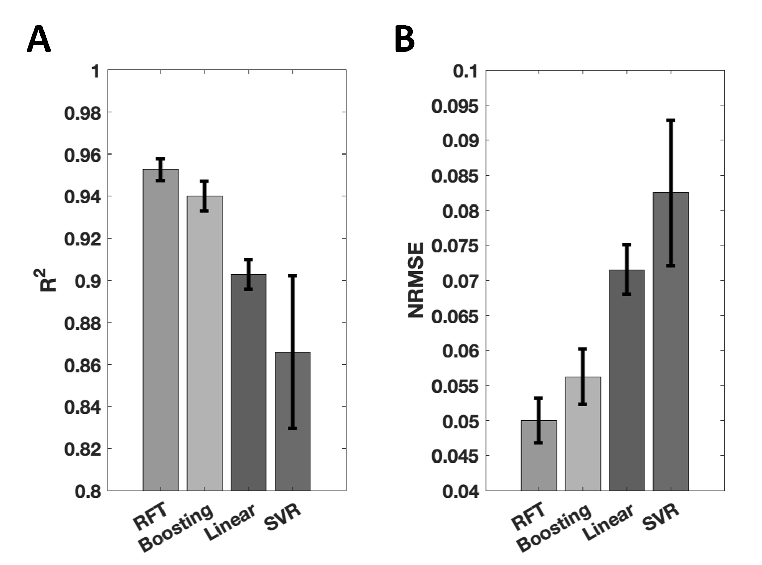
For all methods, model performance was assessed quantitively with leave-one-out cross-validation over 26 subjects, using two metrics – $$$R^2$$$ score and normalised root-mean-squared error (NRMSE):
$$R^2=1-\frac{\sum_i{(\kappa_\mathrm{AFI,i}-\hat{\kappa}_\mathrm{AFI,i})^2}}{\sum_i{(\kappa_\mathrm{AFI,i}-\bar{\kappa}_\mathrm{AFI}})^2}$$
$$\mathrm{NRMSE}=\sqrt{\frac{\sum_i{(\kappa_\mathrm{AFI,i}-\hat{\kappa}_\mathrm{AFI,i})^2}}{\sum_i{(\kappa_\mathrm{AFI,i})^2}}}$$
where $$$i$$$ indexes voxels, $$$\bar{\kappa}_\mathrm{AFI}$$$ is the average observed $$$\kappa_\mathrm{AFI,i}$$$ over all voxels.

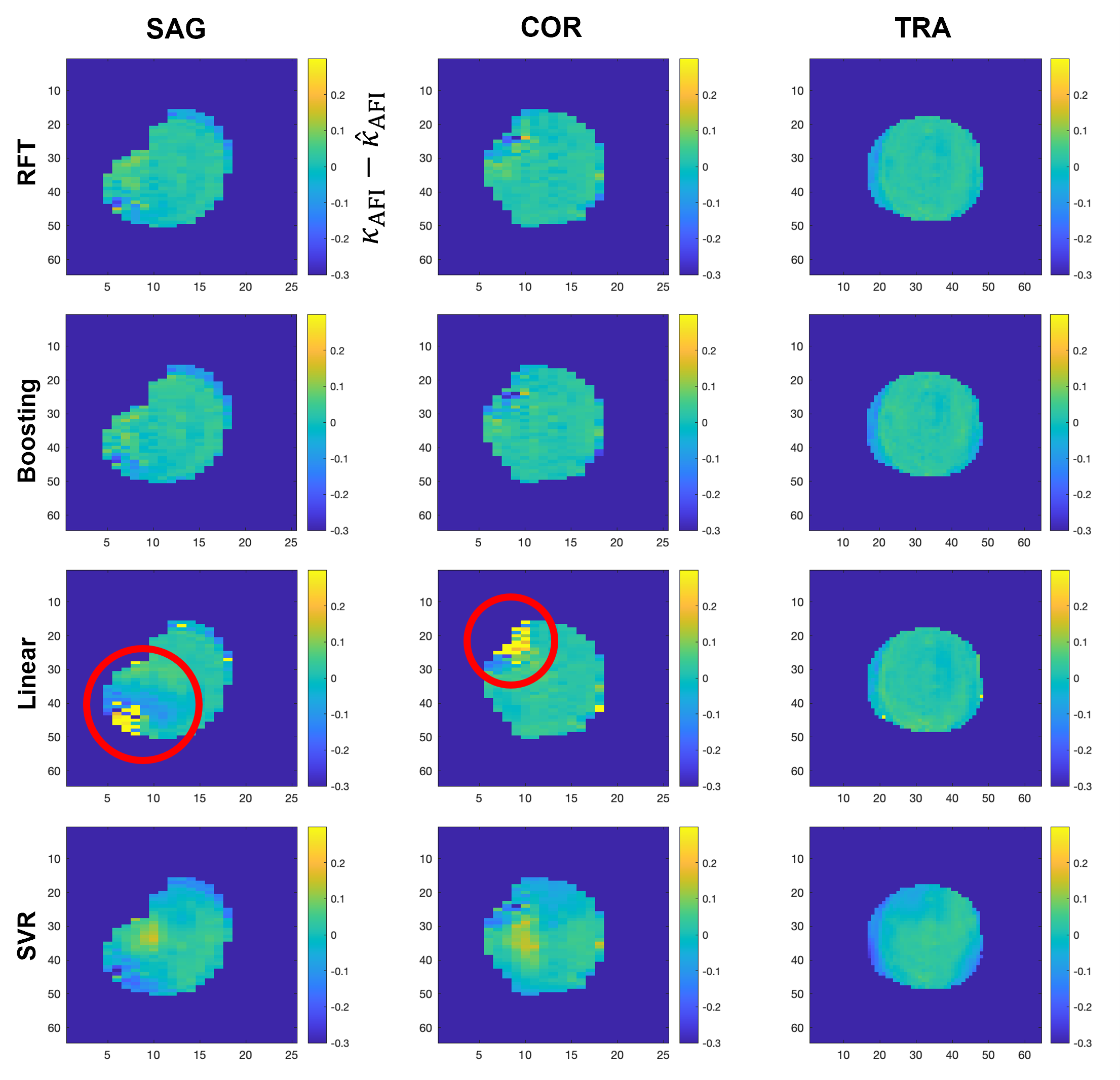
Example maps of the difference between target and prediction were also displayed for visual assessment of all methods. An overfitting study was also performed on the two most successful methods, by comparing the $$$R^2$$$ score obtained when testing on training data to that obtained with cross-validation. The ability of the best method from (ii-iv) to match satTFL to AFI maps across the whole range of FAs was finally compared to that of linear fitting. All computations were performed in MATLAB (The MathWorks, Natick, MA, USA).

Results & Discussion

Quantitative analysis results with the four techniques are presented in Figure 1, in which RFT exhibits the highest $$$R^2$$$ and lowest NRMSE, followed by boosting, linear fitting and finally SVR.

Figure 2 shows a representative case. Difference maps obtained with RFT and boosting show limited deviation from the target, and appear less location-dependent than with linear fitting.

These two methods underwent the overfitting assessment. For RFT, average $$$R^2$$$ score was 0.951 and 0.977 with cross-validation and without, respectively. In contrast, boosting yielded scores of 0.945 and 0.998, respectively. RFT’s smaller $$$R^2$$$ difference than boosting indicates a better resistance to overfitting.

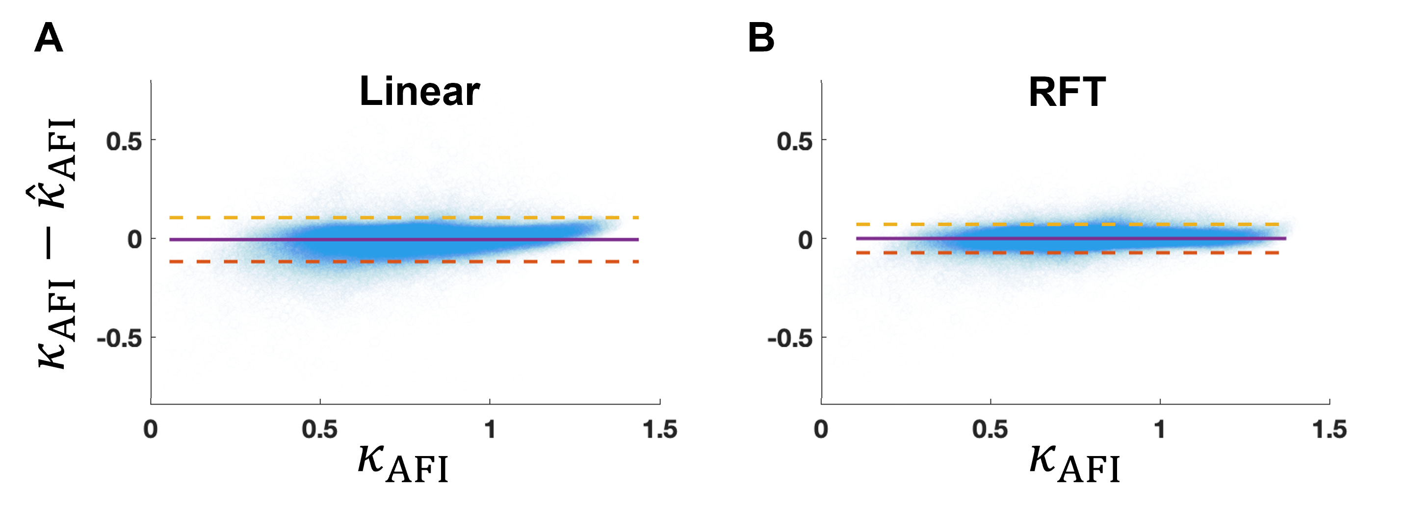
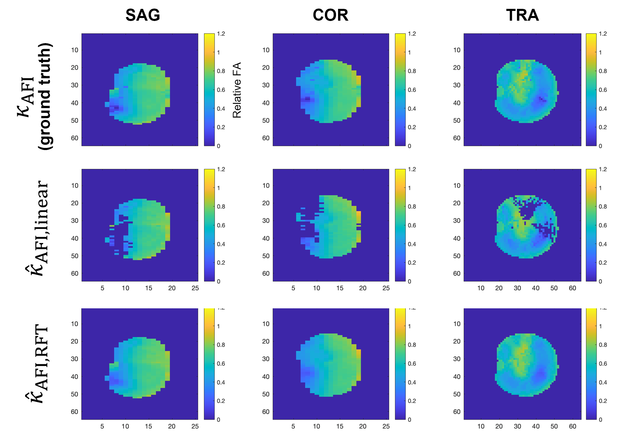
Figure 3 shows that the error between predicted and target $$$B_1^+$$$ from RFT is generally smaller than that from linear fitting. Furthermore, it is more constant across the FA range than linear fitting, which tends to correct high FAs better than small ones. Figure 4 further demonstrates the capacity of the RFT to leverage additional features to interpolate FA from voxels missing from the source satTFL.

Conclusion

We have described a non-linear model that allows calibration of fast-acquired satTFL brain $$$B_1^+$$$ maps to the more accurate but slower AFI maps, in a more reliable way than the previously introduced linear model. While the new correction is more accurate throughout the range of FA values encountered, the effect of the correction is particularly noticeable for lower FAs. Additionally, by accounting for more features than the $$$B_1^+$$$ intensity alone, and especially the spatial locations of voxels, the selected random-forest-based correction provides better calibration across the brain.

Future work includes acquiring more data – which will allow investigating neural-network methods – as well as assessing cases of pathological brains, and implementing the method on the scanner for inline in-vivo testing.

Acknowledgements

This work was supported by a Wellcome Trust collaboration in science award [WT201526/Z/16/Z], by core funding from the Wellcome/EPSRC Centre for Medical Engineering [WT203148/Z/16/Z] and by the National Institute for Health Research (NIHR) Biomedical Research Centre based at Guy’s and St Thomas’ NHS Foundation Trust and King’s College London and/or the NIHR Clinical Research Facility. The views expressed are those of the author(s) and not necessarily those of the NHS, the NIHR or the Department of Health and Social Care.