0934
Minimizing Background Phase in PC-MRI with the Gradient Impulse Response Function (GIRF) and Gradient Optimized (GrOpt) Velocity Encoding1Radiological Sciences Laboratory, Stanford University, Stanford, CA, United States, 2Radiology, Veterans Administration Health Care System, Palo Alto, CA, United States
Synopsis
Keywords: Flow, Velocity & Flow
Background phase errors in PC-MRI flow measurements are caused by eddy currents and mechanical vibrations that produce unwanted magnetic fields, thereby reducing velocity measurement accuracy. In this work, we demonstrate that a GIRF measurement can be used to predict the PC-MRI background phase, then used to design gradient optimized (GrOpt) velocity encoding waveforms that minimize these errors. The method is tested in static phantoms and in vivo, where 4.8x to 6.4x reductions in background velocity are seen. Phantom results showed a reduction from 0.74±0.22 cm/s to 0.15±0.12 cm/s, and in vivo results showed reductions from 0.93±0.10 cm/s to 0.13±0.08 cm/s.
Introduction
Phase contrast MRI (PC-MRI) encodes tissue velocity into the image phase, thereby providing a useful tool for measuring blood flow, among other uses. However, PC-MRI velocity estimates are plagued by background phase errors that reduce measurement accuracy. The problem arises from eddy current fields from the flow encoding bipolar gradients and mechanical vibration-induced fields cause spurious background phase.Background phase corrections are typically done in post-processing, either with a static phantom measurement or with polynomial fitting1,2. Both have some effectiveness, but static phantom measurements require a post-exam calibration scan, and polynomial fitting is prone to limited tissue suitable for fitting and wrap-around artifacts. A prospective method of correction that modifies TE and TR has also recently been proposed3.
In this work, we demonstrate that a gradient impulse response function (GIRF) measurement can be used to predict the background phase (velocity) response in PC-MRI. We use this GIRF measurement to define a background velocity minimization constraint, then design optimal PC-MRI waveforms using the gradient optimization (GrOpt) framework4. Our approach enables the design of arbitrary gradient waveforms that have a predicted background phase (velocity) of zero at the echo time (TE).
Methods
A GIRF measurement was performed in a spherical phantom following the methods described in5. The 0th to 2nd order responses were calculated, however for this work only the 0th order response was used.The GIRF was used to implement an operator that predicts background velocity ($$$BGv_0$$$) based on the measured GIRF, and the target gradient waveform. An overview and description of this process is described in Figure 1, which outlines the prediction of $$$BGv_0$$$. The waveforms can be jointly and numerically optimized using GrOpt so that $$$BGv_0=0$$$ at a specified time (e.g. t=TE).
Fig. 1a shows the 2D PC-MRI gradient waveforms for through-plane velocity encoding (slice-select gradient, bipolar gradient with Venc=160cm/s, and a spoiler gradient with 2π spoiling). The background velocity constraint was set to enforce the predicted $$$BGv_0\leq.05$$$cm/s in a 120µs. Three different minimization window locations (win1 to win3) were evaluated to test if the optimization could be used to reduce background velocity at an arbitrary timepoint, thereby demonstrating flexibility in echo time selection. Six total bi-polar waveform combinations were optimized with GrOpt: 1) for each of the three window positions (win1 to win3); and 2) for bipolar and bipolar + spoiler gradient waveforms. Gradient waveforms and the predicted background velocity are shown in Figure 2.
The waveforms were tested by collecting 40 PC-MRI images in a static phantom, each with different individual TEs (40µs spacing). The sequence was implemented in Pulseq6. All other gradient timings were kept constant except for the positioning of the readout gradient, and therefore the TE. The TR was long (12ms) to accommodate the sliding TE, but could be much shorter in a final implementation. The background velocity was calculated with polynomial fitting, which was then compared to the GIRF predicted background velocity at that TE.
Additionally, the conventional bipolar gradient waveform and two of the optimized waveforms (win1, win1+spoiler) were tested healthy volunteers (N=5) through an axial slice of the liver (IRB approved, consented). A single TE (3.82ms) within the minimization window was acquired in these experiments and background velocity measured.
Results
Figure 2 shows the conventional and optimized waveforms designed for each problem. The additional time needed for each bipolar was 0-190µs compared to the reference bipolar, and no additional spoiling time was used when optimizing the spoilers.Figure 3 shows ten velocity images at different TEs for each optimization. Qualitatively the background velocity is very small within the target windows. Figure 4 shows the measured background velocity as a function of TE, where the measured background velocity is well below the ≤0.6cm/s threshold (an acceptable level as per7) within each minimization window. The mean background velocity in the minimization windows was reduced 4.8-fold from .74±.22 cm/s to .15±.12 cm/s. The Pearson coefficient between the predicted and measured responses was r=0.91.
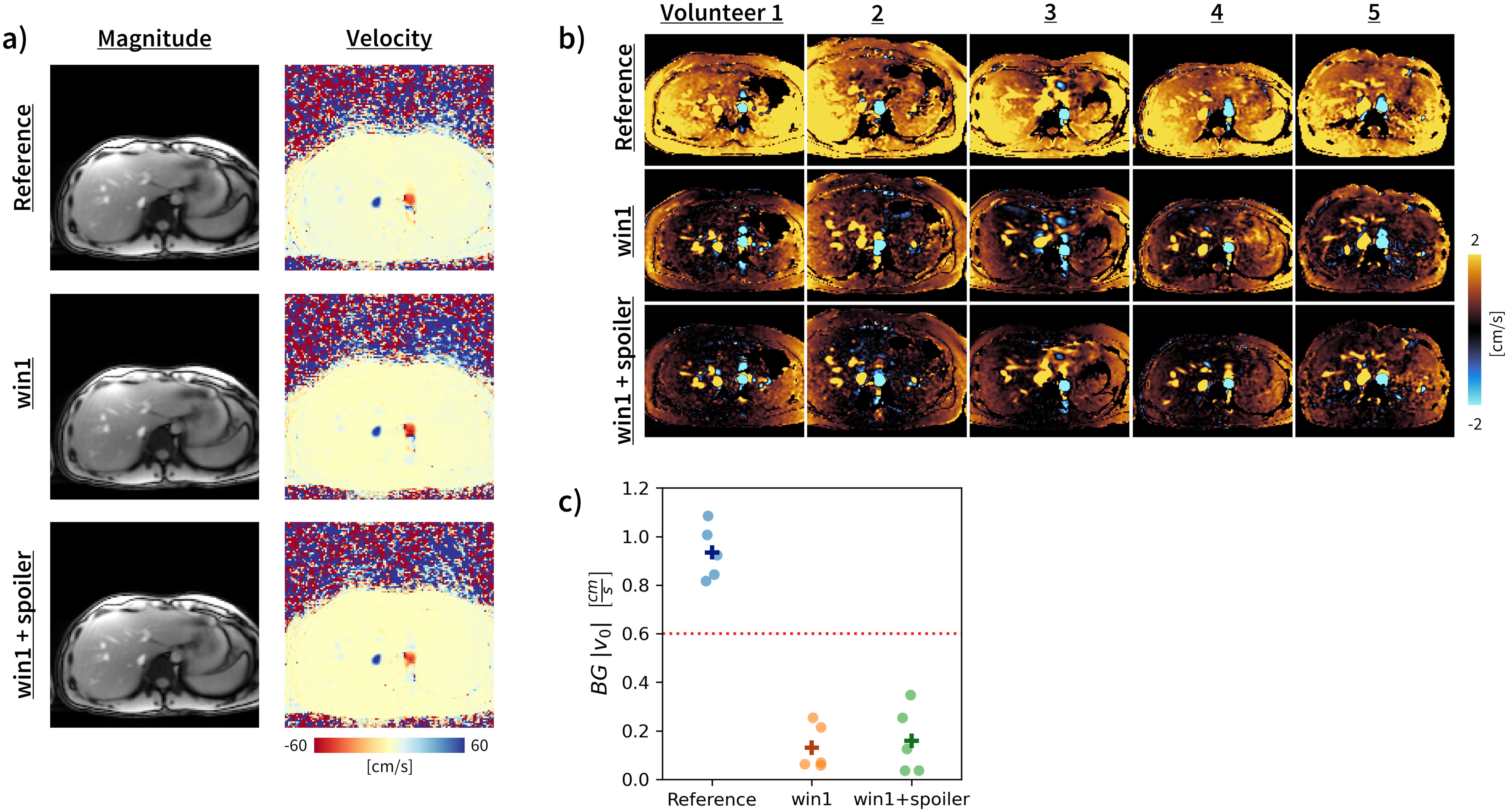
Figure 5 shows in vivo results, where substantially reduced background velocity is evident and reduced 6.4-fold from .93±.19cm/s (reference) to .13±.08cm/s (win1) and .16±.11cm/s (win1+spoiler) across volunteers.
Discussion
In this work, we showed that by using a GIRF and GrOpt we could optimally design gradient waveforms that encoded velocity while significantly reducing background velocity errors to a point where post-processing correction would not be needed. This is achieved with gradient waveforms that are minimally longer (<=190µs) than their conventional comparison (and could potentially be shorter with the addition of other constraints8).As seen in Figure 4, while the measured responses showed very good background velocity reduction, they did not always get as close to zero as predicted. The source of this discrepancy warrants further investigation, and may require a higher SNR GIRF measurement, or perhaps is related to very low frequency components not being measured well with the GIRF9.
For simplicity, only the 0th order GIRF was considered, ignoring higher order responses. Future work will test additional constraints on these spatial responses. Also, only axial slices at isocenter were acquired so the same GIRF could be used in optimization, whereas adjusting the slice orientation and position will necessitate linear combinations of different response functions.
Acknowledgements
NIH R01 HL131823 and HL152256 to DBEReferences
[1] Chernobelsky, A., Shubayev, O., Comeau, C. R. & Wolff, S. D. Baseline correction of phase contrast images improves quantification of blood flow in the great vessels. Journal of Cardiovascular Magnetic Resonance 9, 681–685 (2007).
[2] Walker, P. G. et al. Semiautomated method for noise reduction and background phase error correction in MR phase velocity data. J Magn Reson Imaging 3, 521–530 (1993).
[3] Dillinger, H., Peper, E., Guenthner, C. & Kozerke, S. Background Phase Error Reduction in Phase-Contrast MRI based on Acoustic Noise Recordings. in ISMRM Annual Meeting, Remote (2021).
[4] Loecher, M., Middione, M. J. & Ennis, D. B. A gradient optimization toolbox for general purpose time-optimal MRI gradient waveform design. Magn Reson Med 84, 3234–3245 (2020).
[5] Rahmer, J., Mazurkewitz, P., Börnert, P. & Nielsen, T. Rapid acquisition of the 3D MRI gradient impulse response function using a simple phantom measurement. Magnetic Resonance in Medicine 82, 2146–2159 (2019).
[6] Layton, K. J. et al. Pulseq: a rapid and hardware-independent pulse sequence prototyping framework. Magnetic resonance in medicine 77, 1544–1552 (2017).
[7] Gatehouse, P. D. et al. Flow measurement by cardiovascular magnetic resonance: a multi-centre multi-vendor study of background phase offset errors that can compromise the accuracy of derived regurgitant or shunt flow measurements. Journal of Cardiovascular Magnetic Resonance 12, 5 (2010).
[8] Loecher, M., Magrath, P., Aliotta, E. & Ennis, D. B. Time-optimized 4D phase contrast MRI with real-time convex optimization of gradient waveforms and fast excitation methods. Magnetic Resonance in Medicine 82, 213–224 (2019).
[9] van Gorkum, R. J. H., Guenthner, C., Koethe, A., Stoeck, C. T. & Kozerke, S. Characterization and correction of diffusion gradient-induced eddy currents in second-order motion-compensated echo-planar and spiral cardiac DTI. Magnetic Resonance in Medicine 88, 2378–2394 (2022).
Figures
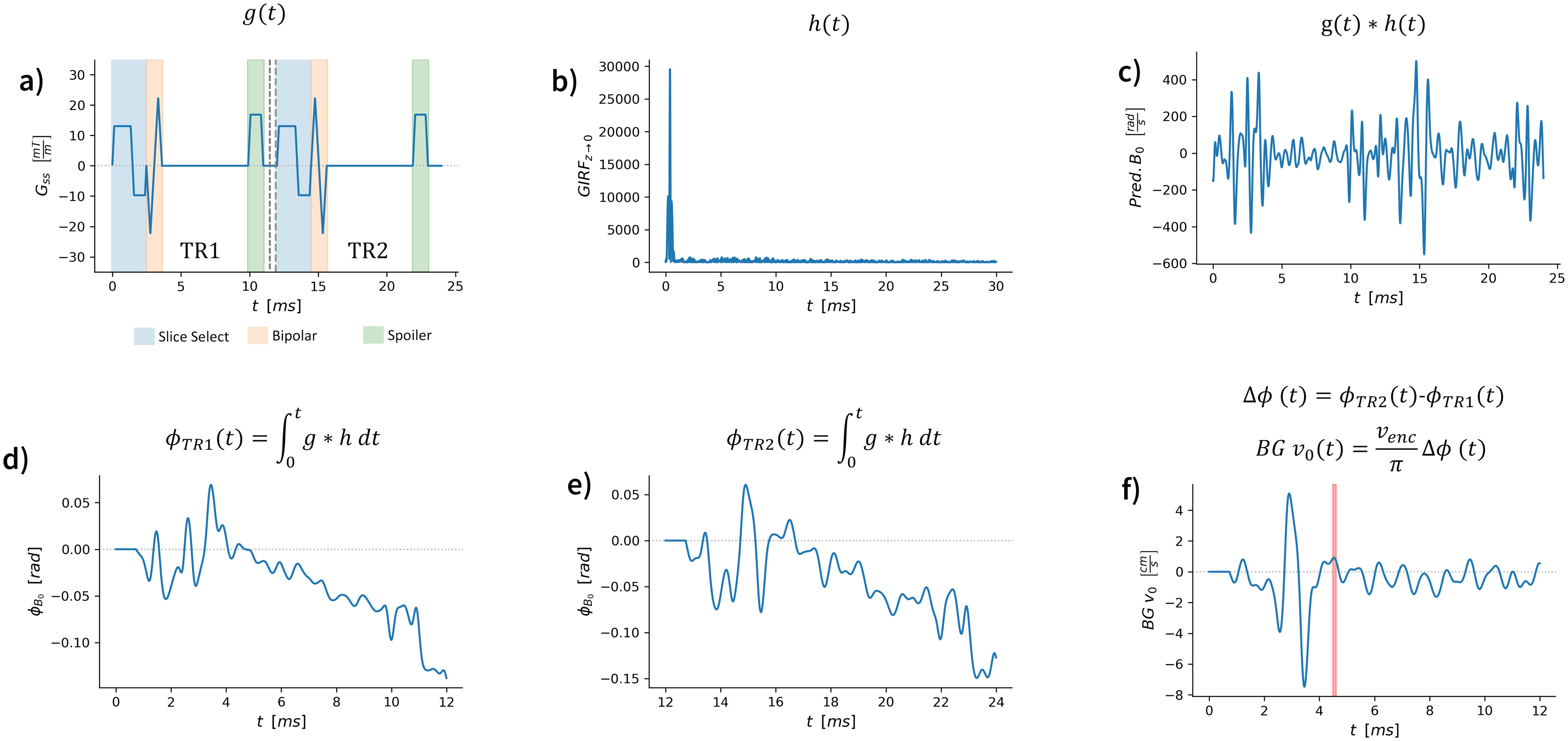
Figure 1: Demonstration of the GIRF-predicted velocity for a bipolar phase-contrast experiment. a) Slice select gradient waveforms, g(t), for two TRs with opposite bipolar velocity encoding. b) measured GIRF, h(t), for zero-order fields. c) convolution of the gradient waveform with the GIRF predicts the field response. d) and e) cumulative phase effect for each individual TR from the time of excitation. f) predicted background velocity after complex differencing and converting to velocity. The red band shows an example of a window around the echo time to be minimized.
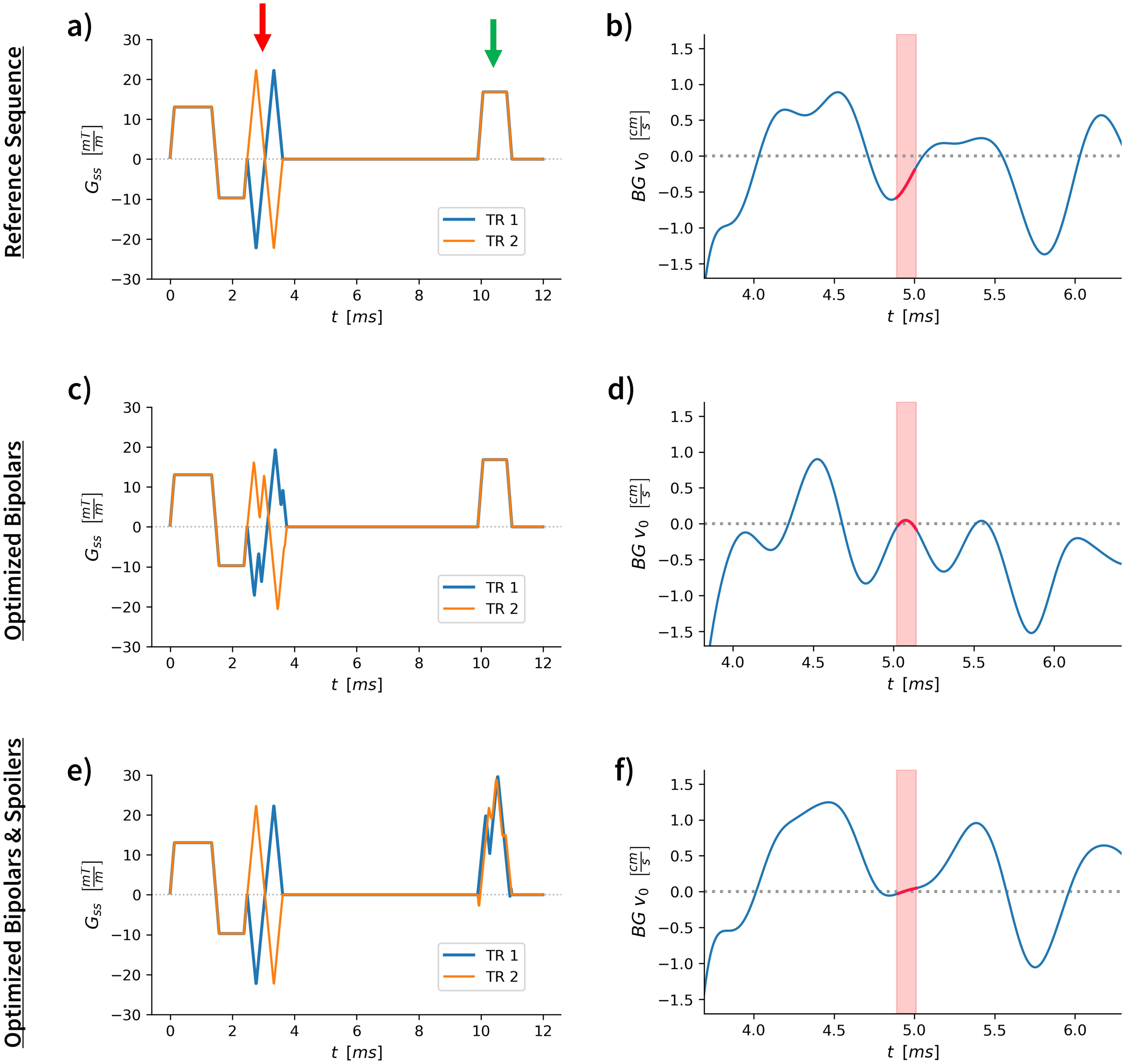
Figure 2: The GrOpt gradient waveform optimization results for the win2 position (a,c,e), and the predicted background velocity for each waveform (b,d,f). Red arrows show bipolars, green arrow show spoilers. The red band shows the minimization window. The top row is for conventional bipolar encoding waveforms, showing the non-zero BGv expected. In the next two rows, the gradient waveforms were optimized to minimize the background velocity within the respective windows. The middle row only optimized the bipolars, and the bottom row optimized both the bipolars and spoilers.
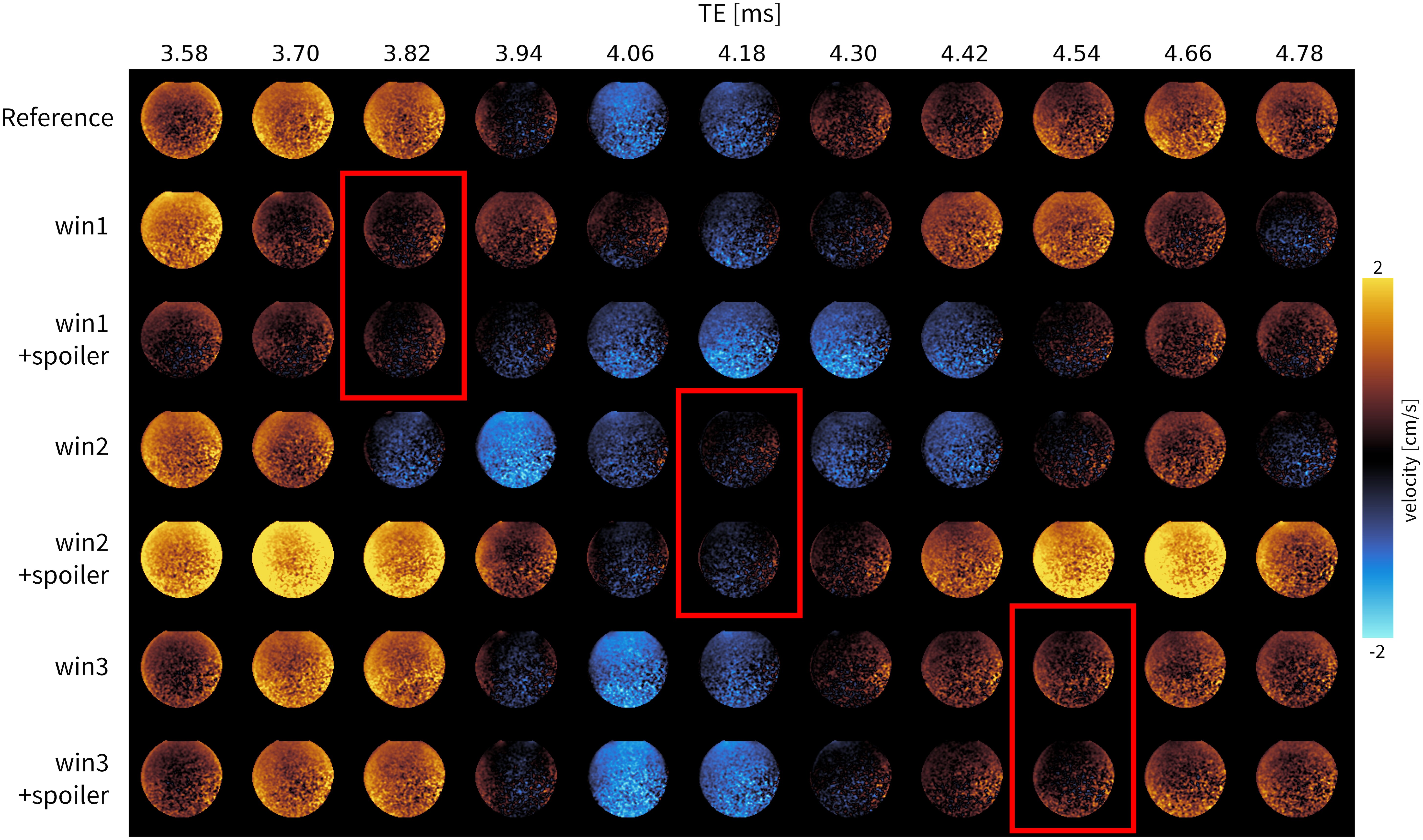
Figure 3: Static phantom velocity maps for different TEs (columns) and a range of PC-MRI gradient waveforms (rows). Only 10 of the 40 TEs acquired are shown. Each row represents a different gradient optimized (GrOpt) waveform. Red boxes highlight velocity maps with echo times that fall within the intended window for which the background velocity approaches zero. Background velocities are generally larger for the other evaluated TEs. When including spoilers in the optimization the response also changes as predicted (Fig 2) and maintains the nulling performance.
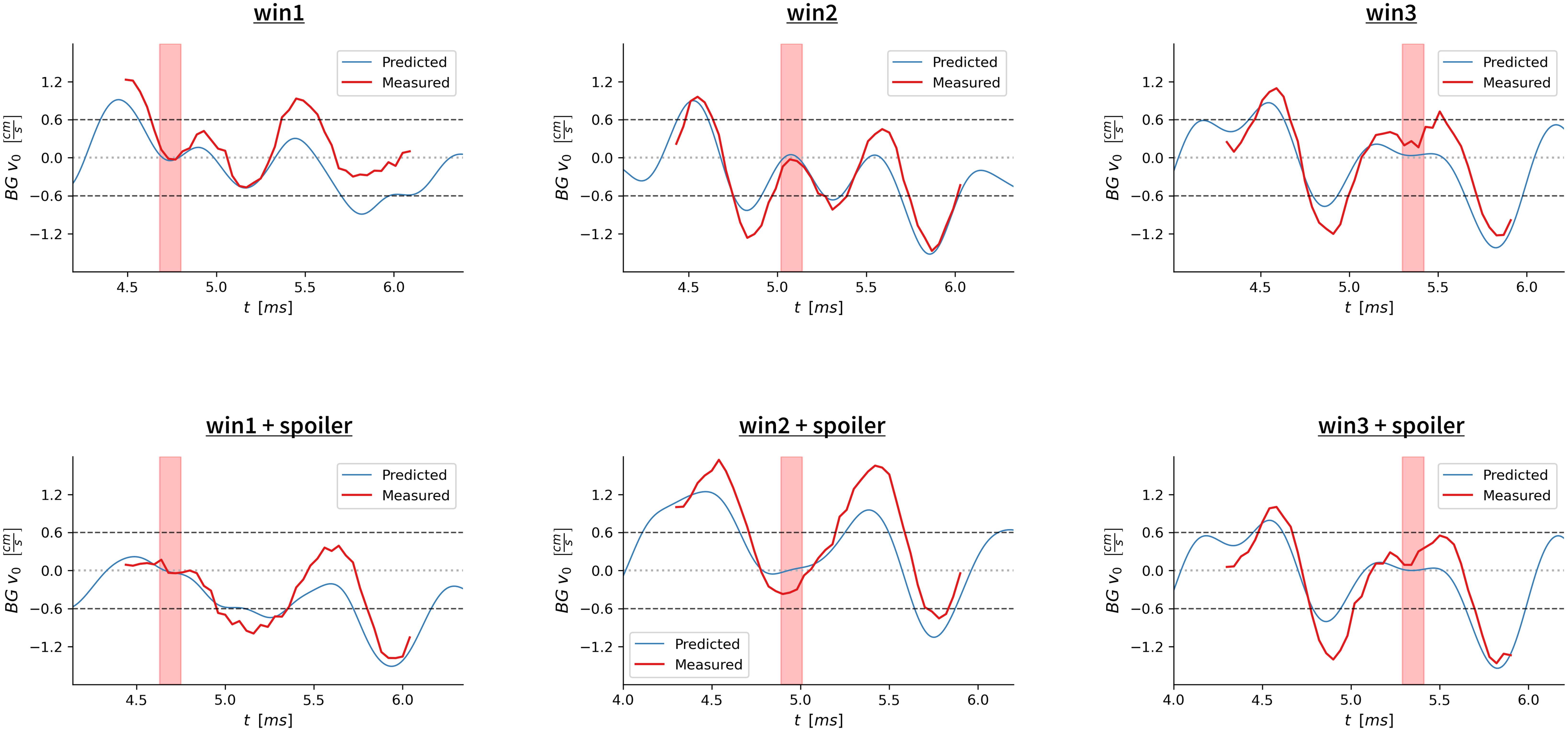
Figure 4: Background velocity in a static phantom from the multi-TE imaging experiment. Red lines are the measured 0th order background velocity across the entire phantom for each TE. The blue line shows the GIRF predicted response. The horizontal dashed lines show the ±0.6 cm/s window for acceptable background velocity offsets [7]. Red bands show the minimization window and demonstrate near zero background velocity offsets for both measured and predicted responses.