0931

Deep learning based segmentation of aortic cross sections (2D+t) in multi-vendor 4D PCMRI

Chiara Manini¹, Markus Hüllebrand^1,2, Marius Pullig³, Titus Kühne^1,4, Sarah Nordmeyer⁵, Lina Jarmatz⁵, Andreas Harloff⁶, Jeanette Schulz-Menger^4,5, and Anja Hennemuth^1,2,4,7
¹Institute of Computer-assisted Cardiovascular Medicine, Charité – Universitätsmedizin Berlin, Berlin, Germany, ²Fraunhofer MEVIS, Bremen, Germany, ³IBM Germany, Berlin, Germany, ⁴DZHK (German Center for Cardiovascular Research), Partner site Berlin, Germany, ⁵Charité – Universitätsmedizin Berlin, Berlin, Germany, ⁶University Hospital Freiburg, Freiburg, Germany, ⁷University Medical Center Hamburg-Eppendorf, Hamburg, Germany

Synopsis

Keywords: Flow, Velocity & Flow, Aorta segmentation

Standardized 4D PCMRI postprocessing protocols could enable comparable bloodflow quantification. We propose an automatic segmentation of aortic cross section over time with a residual trained data from different imaging sequences, scanner types, pathologies and position of cross section planes. Dice score, Hausdorff metric as well as flow and velocity curves for the segmented areas show good performance both in the validation and test sets.

Introduction

4D PCMRI enables comprehensive assessment of aortic bloodflow, and medical societies suggest standardized postprocessing protocols to enable comparative quantitative analysis. Data acquired with different protocols, scanners and sequences can differ regarding intensity ranges and velocity encoding. Existing approaches for 3D and 4D segmentation of 4D PCMRI data achieve good results for specific imaging sequences and scanner manufacturers [1-3]. The authors propose a multi-site ML model for automatic segmentation of aorta cross sections over time and evaluate the results in terms of accuracy of segmentation masks and the effect of segmentation differences on derived clinical parameters such as throughflow.

Methods

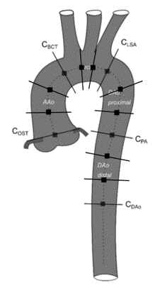
We considered 4D-flow MRI data from 205 subjects; 130 without known aortic pathology (Siemens Trio Tim 3T) [4], 59 with aortic stenosis (Philips Achieva 1.5T) [5], and 8 healthy volunteers (Siemens Prisma Fit 3T, Philips Ingenia 3T) [6]. Per dataset 11-12 planes (Figure 1) were placed perpendicular to the aortic centerline obtaining a total number of 2316 cross sections, and lumen boundaries were annotated by medical experts (21 to 57 frames/cardiac cycle depending on the heart rate).
A residual Unet [7] was trained to generate 3D aortic cross sectional segmentations (x,y,t) on preprocessed (phase unwrapping, offset correction) 4D flow MRI data. 2D+t planes of magnitude and velocities fields were prepared for processing as follows:

Z-score normalization
Spatiotemporal resampling to obtain a final in-plane resolution of 1.54 mm2 and 64 timesteps
Padding/cropping to an in-plane dimension of 64x64
Concatenation of magnitude and velocity fields as channels.

A composite loss function (cross entropy and Dice) was used during training. A sigmoid function generates probabilities per voxel, which are thresholded with 0.5. The model was implemented in Python 3.7.6 using monai 0.8.1. Training and testing were performed on an AMD EPYC 7302 16-Core Processor with a Nvidia A40 GPU. Dice score (DS) and Hausdorff Distance (HD) were computed with monai 0.8.1. On the test set we computed flow I(t) and velocity v(t) curve as:
$$v(t) = \frac{1}{\mid A(t)\mid} \int_{A(t)}^{}\parallel v(x,y,t)\parallel dA$$
$$I(t) = \int_{A(t)}^{} <v(x,y,t),n>dA$$
With:

||v|| the magnitude of the velocity vector
v(x,y,t) the velocity vector in the point (x,y) at time t
|A(t)| the area of the segmentation on timeframe t
n normal vector of the cross-sectional plane
And <a,b> denotes the scalar product between the vectors a and b

Results

The data were randomly divided into 88% for training, 10% for validation and 2% for testing (see Figure 1). DS and HD were:

Validation set: DS = 0.89±0.04, HD = 2.99±1.89
Test set: DS = 0.89±0.12, HD = 3.95±2.17.

Flow and velocity curves were computed for exemplary cross sections, results are shown in Figure 3, Figure 4 and Figure 5 (best case, exemplary and worst one respectively). In general, the model tends to underestimate the vessel area, but the effect on the flow and velocity curves is minimal (Figure 2 and Figure 3). For the case with lower DS the opposite trend for the segmentation contours is observed (Figure 4). The model segmentation results in a higher throughflow. The manual segmentation might have missed low flow regions.

Discussion

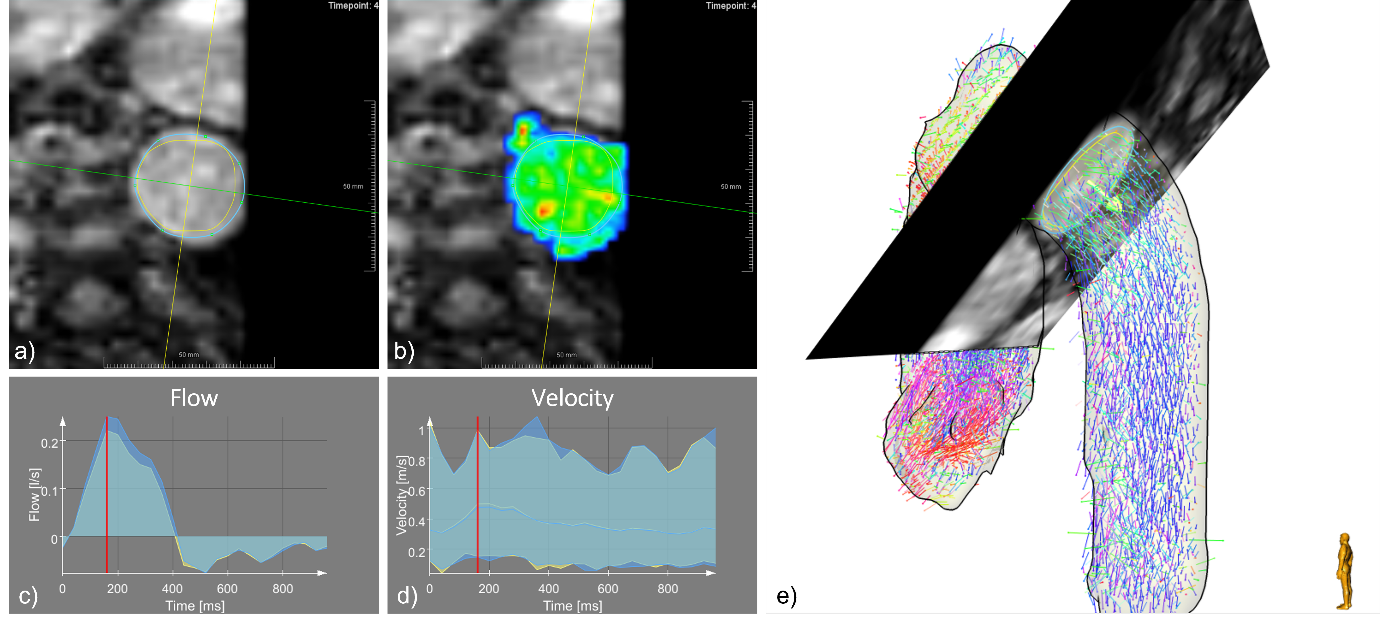
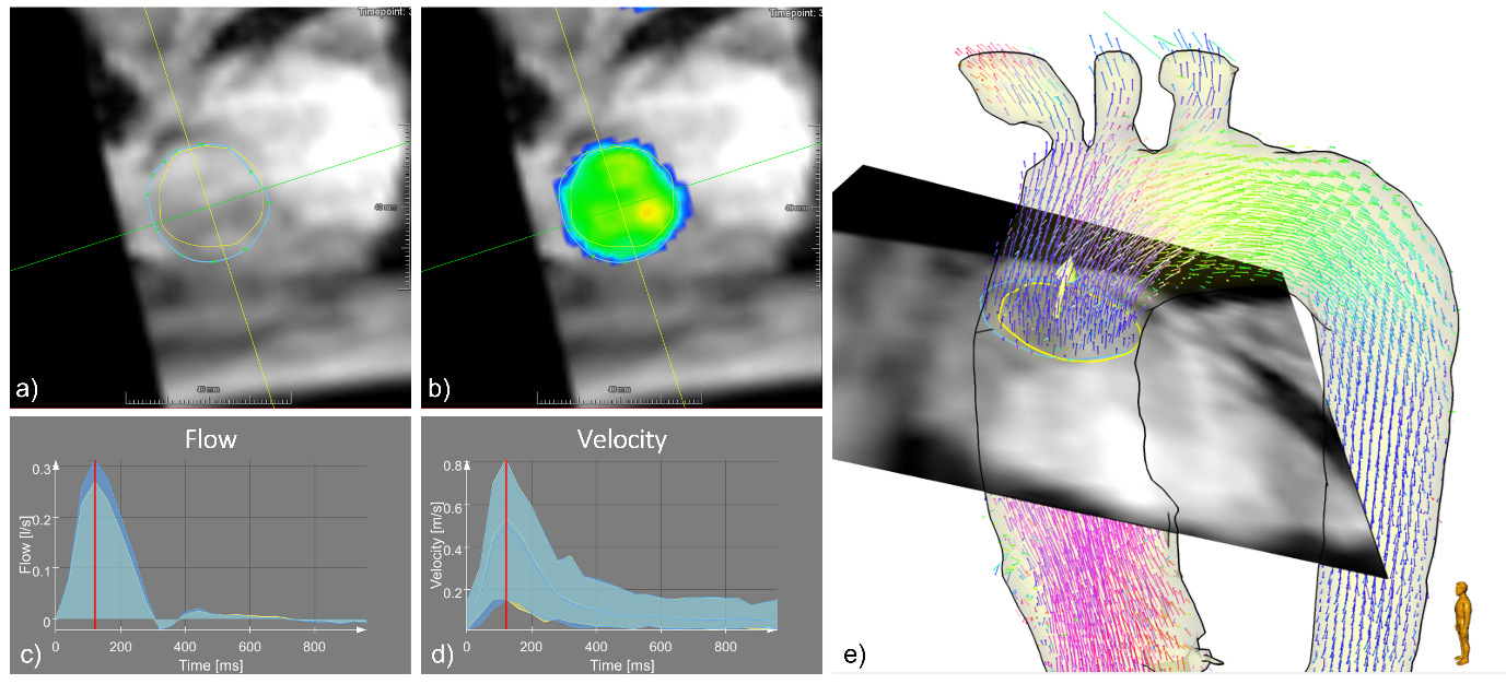
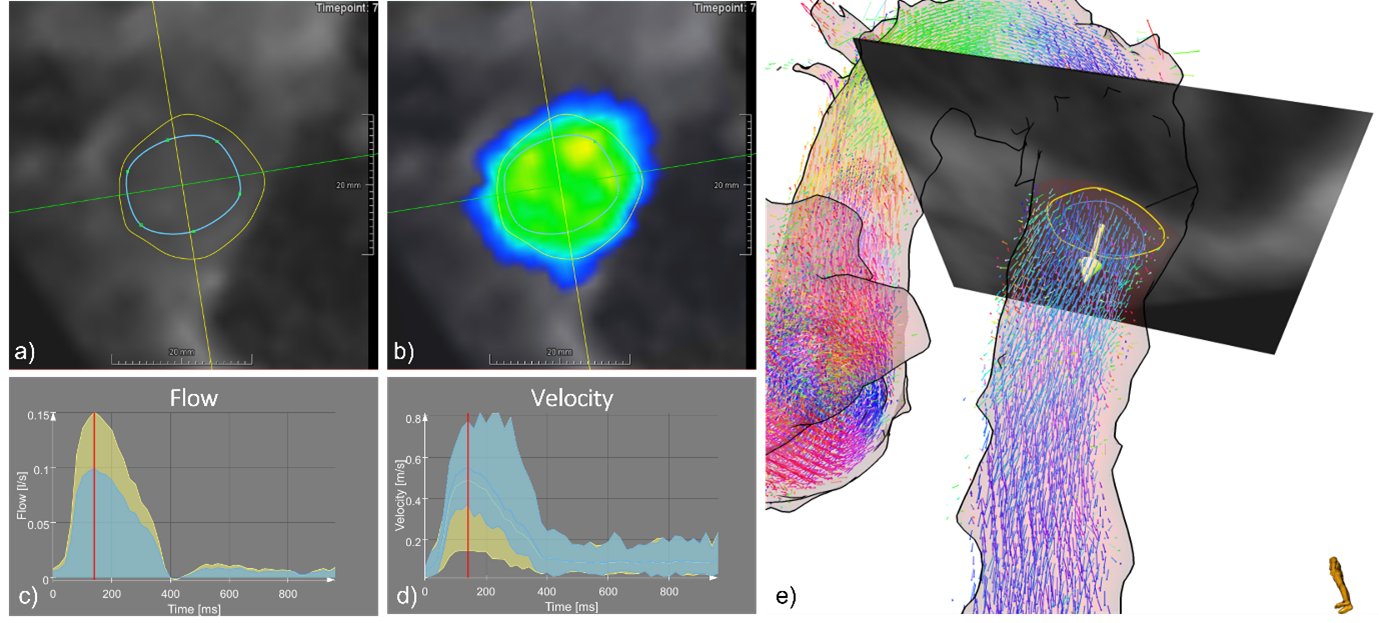
The 3D Unet trained on the multi-scanner, multi-sequence dataset showed good performance for the different manufacturers, pathologies, and cross section positions for all age groups (21-81). The automatic segmentation provided flow and velocity curves comparable with expert analyses. The inspection of cases with lower DS indicates that the model might perform better than the expert in low contrast regions (Figure 4).

Conclusion

With a multicenter, multiscanner, multisequence dataset it might be possible to provide automatized segmentation methods, which enable comparable measurements on 4D flow datasets acquired in different scenarios.

Acknowledgements

Funding from the German Research Foundation (GRK2260, BIOQIC).

Funding by the German Research Foundation (DFG) as part of SFB-1470, B06.

References

[1] Berhane H, Scott M, Elbaz M, Jarvis K, McCarthy P, Carr J, Malaisrie C, Avery R, Barker AJ, Robinson JD, Rigsby CK, Markl M. Fully automated 3D aortic segmentation of 4D flow MRI for hemodynamic analysis using deep learning. Magn Reson Med. 2020 Oct;84(4):2204-2218. doi: 10.1002/mrm.28257.

[2] Pradella M, Scott MB, Omer M, Hill SK, Lockhart L, Yi X, Amir-Khalili A, Sojoudi A, Allen BD, Avery R, Markl M. Fully-automated deep learning-based flow quantification of 2D CINE phase contrast MRI. Eur Radiol. 2022 Oct 29. doi: 10.1007/s00330-022-09179-3.

[3] Bustamante, M., Viola, F., Engvall, J., Carlhäll, C.-J. and Ebbers, T. (2022), Automatic Time-Resolved Cardiovascular Segmentation of 4D Flow MRI Using Deep Learning. J Magn Reson Imaging. https://doi.org/10.1002/jmri.28221

[4] Harloff A, Hagenlocher P, Lodemann T, Hennemuth A, Weiller C, Hennig J, Vach W. Retrograde aortic blood flow as a mechanism of stroke: MR evaluation of the prevalence in a population-based study. Eur Radiol. 2019 Oct;29(10):5172-5179. doi: 10.1007/s00330-019-06104-z.

[5] Nordmeyer S, Lee CB, Goubergrits L, Knosalla C, Berger F, Falk V, Ghorbani N, Hireche-Chikaoui H, Zhu M, Kelle S, Kuehne T, Kelm M. Circulatory efficiency in patients with severe aortic valve stenosis before and after aortic valve replacement. J Cardiovasc Magn Reson. 2021 Mar 1;23(1):15. doi: 10.1186/s12968-020-00686-0. PMID: 33641670; PMCID: PMC7919094.

[6] Demir A, Wiesemann S, Erley J, Schmitter S, Trauzeddel RF, Pieske B, Hansmann J, Kelle S, Schulz-Menger J. Traveling Volunteers: A Multi-Vendor, Multi-Center Study on Reproducibility and Comparability of 4D Flow Derived Aortic Hemodynamics in Cardiovascular Magnetic Resonance. J Magn Reson Imaging. 2022 Jan;55(1):211-222. doi: 10.1002/jmri.27804. Epub 2021 Jun 25. PMID: 34173297.

[7] Anita Khanna, Narendra D. Londhe, S. Gupta, Ashish Semwal, A deep Residual U-Net convolutional neural network for automated lung segmentation in computed tomography images, Biocybernetics and Biomedical Engineering,Volume 40, Issue 3,2020,Pages 1314-1327,ISSN 0208-5216, https://doi.org/10.1016/j.bbe.2020.07.007.

Figures

Figure 1: Positions of cross sections with annotations. Cost is positioned above the coronary ostia, Cbct is placed before the brachius cephalicus, Clsa is placed after the subclavian artery, Cpa above the pulmonary artery, and Cdao at the diaphragm. The other cross sections in ascendending and descending aorta are placed between the landmark planes with equal spacing. In the arch, additional planes are placed between the branches.

Figure 2: Data overview

Figure 3: Predicted and manual segmentation contour and curves for the best case (DS=0.96). The manual segmentation (light blue) and the predicted one (yellow) are shown on the magnitude image (a), the heatmap for the flow in the cross-section area is shown in the peak flow frame (b). The flow and velocity curve computed on the manual and predicted segmentation are shown in (c) and (d), the red line highlight the visualized timeframe. The vector field within the aorta is shown with the reference plane in the descending aorta (e).

Figure 4: Predicted and manual segmentation contour and curves for an exemplary case (DS=0.83). The manual segmentation (light blue) and the predicted one (yellow) are shown on the magnitude image (a), the heatmap for the flow in the cross-section area is shown in the peak flow frame (b). The flow and velocity curve computed on the manual and predicted segmentation are shown in (c) and (d), the red line highlight the visualized timeframe. The vector field within the aorta is shown with the reference plane in the ascending aorta (e).

Figure 5: Predicted and manual segmentation contour and curves for the worst case (DS=0.697). The manual segmentation (light blue) and the predicted one (yellow) are shown on the magnitude image (a), the heatmap for the flow in the cross-section area is shown in the peak flow frame (b). The flow and velocity curve computed on the manual and predicted segmentation are shown in (c) and (d), the red line highlight the visualized timeframe. The vector field within the aorta is shown with the reference plane in the descending aorta (e).

Proc. Intl. Soc. Mag. Reson. Med. 31 (2023)

0931

DOI: https://doi.org/10.58530/2023/0931