0906
An Analytic Solution for the Modified WASABI Method: Application to Simultaneous B0, B1 and T1 Mapping and Correction of CEST MRI1Physikalisch-Technische Bundesanstalt (PTB), Braunschweig and Berlin, Germany, 2Institute for Neuroradiology, University Hospital Erlangen, Friedrich-Alexander Universität Erlangen-Nürnberg, Erlangen, Germany
Synopsis
Keywords: CEST & MT, Data Processing
CEST MRI provides a contrast sensitive to exchange processes between solute and water protons that was proven to add value in clinical MRI. However, the contrast is susceptible to B0- and B1 field inhomogeneities as well as the T1 relaxation time. Here we present an analytical solution for a modified WASABI method that enables the quantitative mapping of all three parameters simultaneously from a single CEST-like MRI scan. We show that the generated parameter maps and reference maps match well and demonstrate their applicability for the B0, B1 and T1 correction of CEST MRI data.Introduction
A major challenge in CEST MRI is its dependency on B0- and B1-field inhomogeneities, the T1 relaxation time and on experimental settings like saturation time and relaxation delays. In order to ensure accurate and reproducible CEST quantification, all these influences need to be corrected for during post-processing. Correction methods and metrics for the correction of B0, B1 and T1 are widely used in CEST MRI already1–3. Recently, the QUASS-CEST4 method has been proposed that allows to compensate for the influence of the saturation settings. However, all these methods require accurate parameter maps of B0, B1 and especially T1. Here, we show that an analytical form instead of previously proposed neural networks5 can be used to obtain these maps efficiently from a single modified WASABI2,5 scan avoiding the black box character of the NN-based approaches. Finally, we demonstrate its applicability for the correction of CEST MRI data.Methods:
The frequency offset and recover time pattern of a previously modified version of the WASABI method2,5 was further optimized. A novel analytical form based on Mulkern et. al.6 for this “WASABITI” method was derived and implemented in Python. It is not written down here for the sake of brevity. WASABITI (acquisition time 115 s) , CEST, and reference (WASABI for B0 & B1, saturation recovery for T1) scans of six model solutions were acquired on a 3T whole body MRI scanner. The pH was adjusted to 7.0 and creatine concentration to 100 mM for all solutions. The T1 relaxation times were varied using different concentrations of a Gadolinium-based contrast agent (GBCA) aiming for T1 times of 0.75, 1.0, 1.25, 1.5, 2.0 and 2.5 s. WASABITI B0, B1 and T1 mapping was also demonstrated in a healthy volunteer. All MRI sequences were implemented using the open-source (Py)Pulseq framework7,8. Data post-processing was performed in Python using established methods for ∆B0, B1 and T1 correction.1,3,9Results
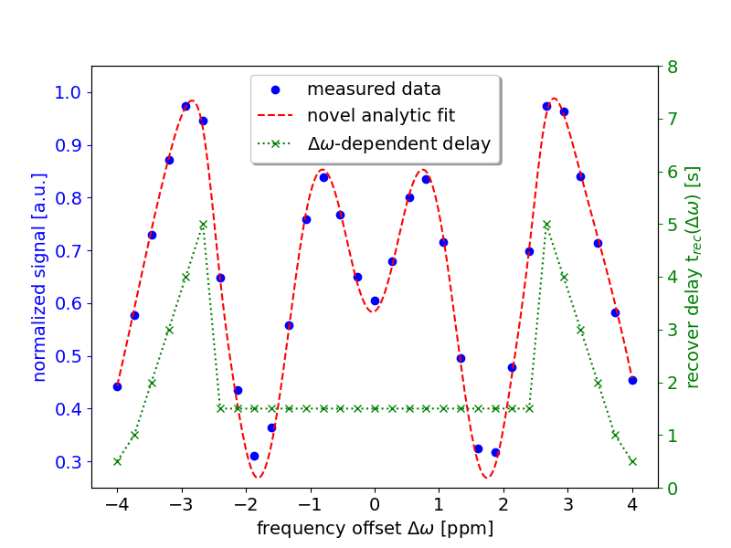
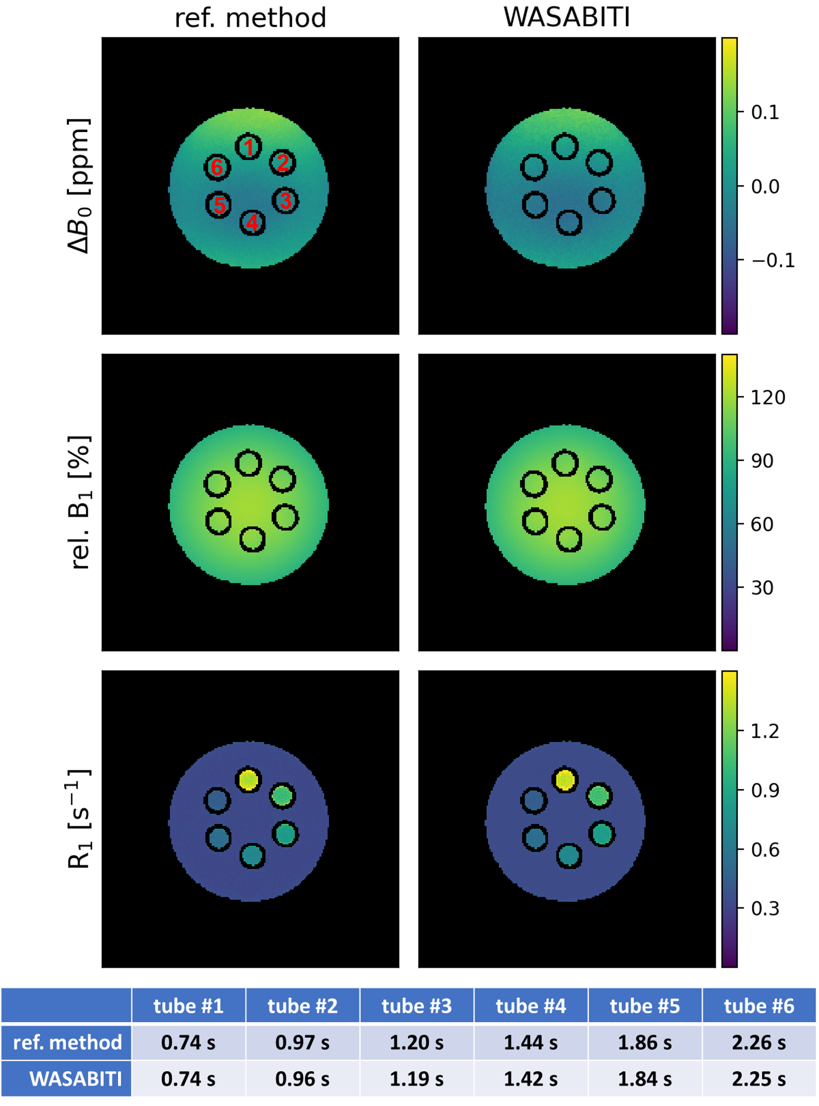
Different frequency offset (∆ω) and ∆ω-dependent recover delay (trec(∆ω)) schemes were investigated. The ∆ω range was increased from ±2 to ±4 compared to previous settings while keeping the total number of offsets (n=31) fixed. An exemplary WASABITI spectrum with corresponding best performing trec(∆ω) scheme, and the well matching least-square fit is shown in figure 1.Figure 2 shows the parameter maps for ∆B0, B1 and R1 generated using the WASABITI method and the corresponding reference maps for a phantom containing six model solutions. All maps match very well. The quantitative ROI-averaged T1 values for the six tubes are summarized below the maps. All deviations from reference values are below 2%.
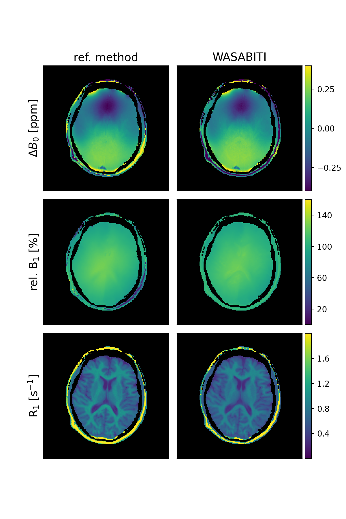
Figure 3 shows the WASABITI and reference parameter maps for the in-vivo brain scan of a healthy volunteer. As in the in-vitro case, all WASABITI and reference maps match well.
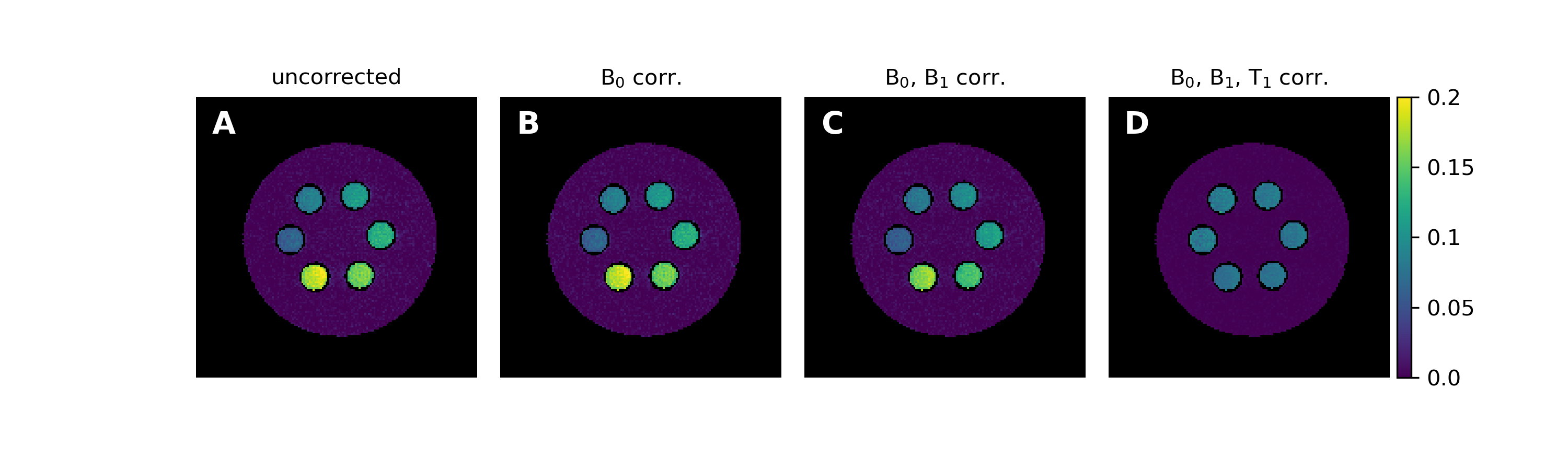
The application of the WASABITI parameter maps to the correction of CEST MRI measurements of the phantom from figure 2 is shown in figure 4. Despite matching creatine concentrations and pH values, the uncorrected CEST contrast (Fig. 4A) shows strong deviations within and especially between the different tubes. The ∆B0 and B1 corrections (Fig. 4B/C) increase the homogeneity within the individual tubes, but variations between the tubes remain. These are eliminated after the T1 correction using the AREX3 metric finally providing equal CEST effects in all tubes independent of B0, B1 or T1.
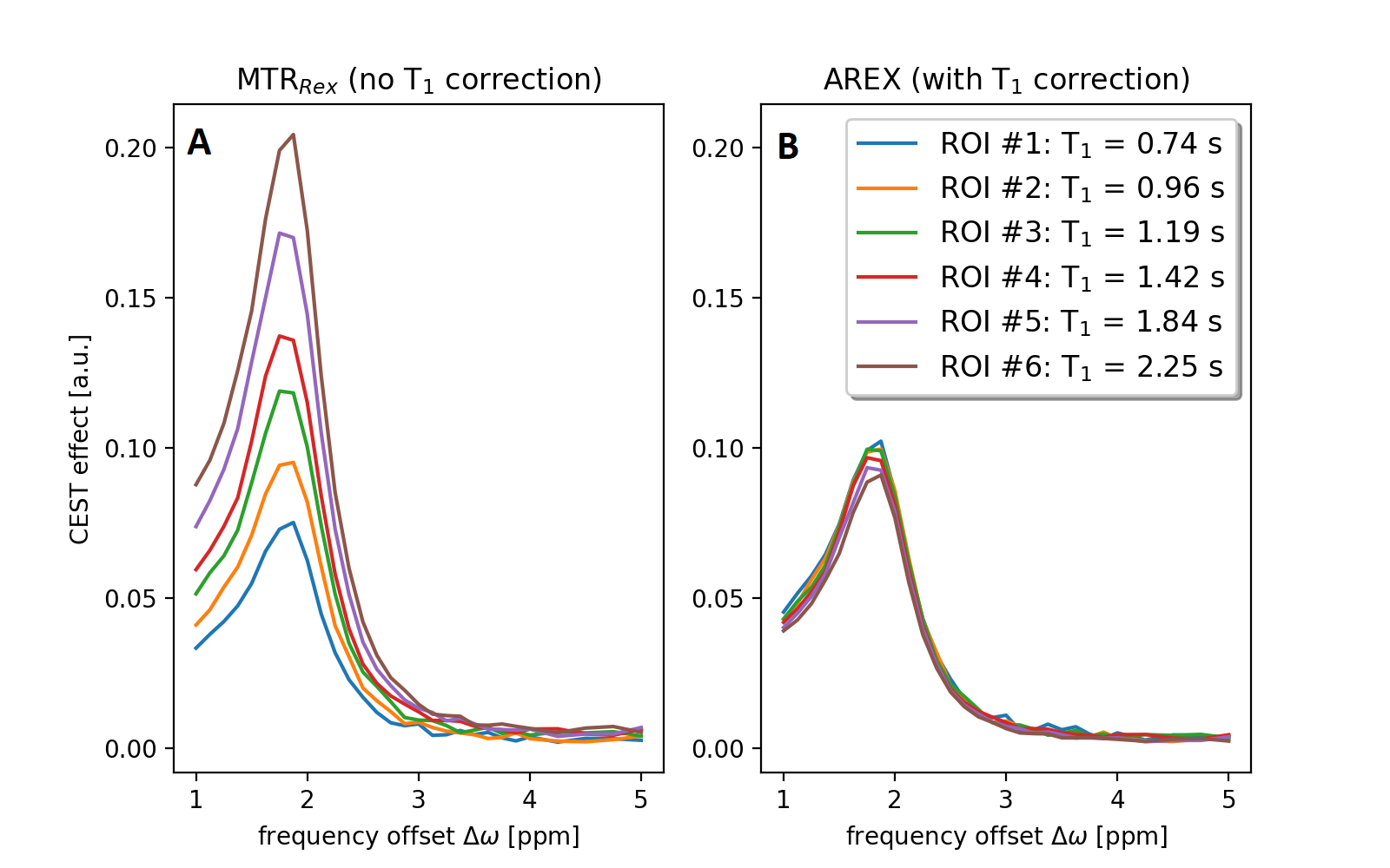
The influence of the T1 correction (using the T1 map from the WASABITI method) on the ROI-averaged, spillover and B1-corrected CEST spectra is shown in figure 5. Without T1 correction, the maximum CEST contrast at 1.9 ppm for the six different tubes varies between 0.07 and 0.21 (Fig. 5A). After T1 correction, the variations are drastically reduced to a range between 0.09 and 0.10 (Fig. 5B).
Discussion
We demonstrated that the presented optimized WASABITI protocol and proposed post-processing enables the simultaneous and accurate mapping of B0, B1 and T1 without additional acquisition time compared to the original WASABI method. The proposed analytical form overcomes the burden of the implementation and training of previously suggested neural networks5. More important, the analytic form increases the flexibility regarding the choice of frequency offsets, recover delays, and total number of acquisition points and enables the straightforward implementation in existing scientific and commercial CEST post-processing software.All predicted parameter maps agree well with the reference maps, both in-vitro and in-vivo. The utilization of these parameter maps in established correction methods1,3,9 led to clear homogeneity improvements within and between the different tubes of the investigated phantom. The good match of all B0, B1 and T1 corrected CEST spectra (Fig. 5B) is an intrinsic accuracy validation of the predicted parameters. Remaining minor differences in the spectra might result from inaccuracies during preparation of the model solutions and potential influences of the varying GBCA concentrations on the exchange rate.
Conclusion
The similarity between the proposed WASABITI sequence and conventional CEST-sequences enables quantitative mapping of B0, B1 and T1 in 3D in less than two minutes when using optimized 3D readouts like Snapshot-CEST10. The additional prediction of T1 is important for both, relaxation compensated CEST and QUASS-CEST, and thus represents an important contribution towards widespread accurate and reproducible CEST MRI.Acknowledgements
This research was funded by the Deutsche Forschungsgemeinschaft (DFG, German Research Foundation) – Grant No. 446320579, 372486779.References
1. Kim M, Gillen J, Landman B a, Zhou J, van Zijl PCM. Water saturation shift referencing (WASSR) for chemical exchange saturation transfer (CEST) experiments. Magn. Reson. Med. 2009;61:1441–50 doi: 10.1002/mrm.21873.
2. Schuenke P, Windschuh J, Roeloffs V, Ladd ME, Bachert P, Zaiss M. Simultaneous mapping of water shift and B1 (WASABI)-Application to field-Inhomogeneity correction of CEST MRI data. Magn. Reson. Med. 2017;77:571–580 doi: 10.1002/mrm.26133.
3. Zaiss M, Xu J, Goerke S, et al. Inverse Z-spectrum analysis for spillover-, MT-, and T1 -corrected steady-state pulsed CEST-MRI--application to pH-weighted MRI of acute stroke. NMR Biomed. 2014;27:240–52 doi: 10.1002/nbm.3054.
4. Sun PZ. Quasi-steady state chemical exchange saturation transfer (QUASS CEST) analysis-correction of the finite relaxation delay and saturation time for robust CEST measurement. Magn. Reson. Med. 2021;85:3281–3289 doi: 10.1002/mrm.28653.
5. Schuenke P, Heinecke K, Narvaez GH, Zaiss M, Kolbitsch C. Simultaneous Mapping of B0, B1 and T1 Using a CEST-like Pulse Sequence and Neural Network Analysis. In: Proc. Intl. Soc. Mag. Reson. Med. 30. London; 2022. p. 2714.
6. Mulkern R V, Williams ML. The general solution to the Bloch equation with constant rf and relaxation terms: application to saturation and slice selection. Med. Phys. 1993;20:5–13 doi: 10.1118/1.597063.
7. Layton KJ, Kroboth S, Jia F, et al. Pulseq: A rapid and hardware-independent pulse sequence prototyping framework. Magn. Reson. Med. 2017;77:1544–1552 doi: 10.1002/mrm.26235.
8. Ravi K, Geethanath S, Vaughan J. PyPulseq: A Python Package for MRI Pulse Sequence Design. J. Open Source Softw. 2019;4:1725 doi: 10.21105/joss.01725.
9. Windschuh J, Zaiss M, Meissner J-E, et al. Correction of B1-inhomogeneities for relaxation-compensated CEST imaging at 7 T. NMR Biomed. 2015;28:529–37 doi: 10.1002/nbm.3283.
10. Zaiss M, Ehses P, Scheffler K. Snapshot-CEST: Optimizing spiral-centric-reordered gradient echo acquisition for fast and robust 3D CEST MRI at 9.4 T. NMR Biomed. 2018;31:e3879 doi: 10.1002/nbm.3879.
Figures