Synopsis

Keywords: Image Reconstruction, Quantitative Susceptibility mapping

We propose a robust Bayesian approach with built-in parameter estimation for quantitative susceptibility mapping (QSM). From a Bayesian perspective, wavelet coefficients of the susceptibility map are modeled by Laplace distribution. Noise is modeled by a two-component Gaussian-mixture distribution, where the second component is reserved to model the noise outliers. The susceptibility map and distribution parameters are jointly recovered using approximate message passing (AMP). The proposed approach achieves better performance in challenging cases of brain hemorrhage and calcification. It automatically estimates the parameters, which avoids subjective bias from the usual visual-tuning step of in vivo reconstruction.

Introduction

QSM is widely used to study iron deposition in the brain, or pathologies such as hemorrhage and calcification [1]. The local field map is first obtained from unwrapped MR phase images. Recovery of the susceptibility map $$$\chi$$$ from the local field map is known as the dipole inversion, it is an ill-posed inverse problem due to the zeros in the dipole kernel along the magic angle. In this case sparse prior information about the susceptibility map is often used to improve the image quality. Regularization approaches like TV-minimization use a parameter $$$\lambda$$$ to balance the trade-off between the data-fidelity term and the regularization term. In practice, visual fine-tuning is typically used to find working parameters or double-check pre-tuned parameters for in vivo reconstructions [2]. However, it also introduces subjective bias to the results inevitably. Additionally, phase unwrapping errors also make the problem challenging. The erroneous phase jumps in the phase image lead to severe streaking artifacts in QSM when a linear least-squares data-fidelity term is used. In order to handle these phase jumps, Liu et al. mapped the local fields to the complex domain via the complex exponential function, and proposed a nonlinear least-squares data-fidelity term that was much more robust [3]. Both the linear and nonlinear least-squares data-fidelity terms imply that the corresponding noise is modeled as additive white Gaussian noise (AWGN). However, in cases that involve brain hemorrhage or calcification, the resulting noise can be better modeled by long-tailed distributions such as the Laplace distribution and the Gaussian-mixture distribution. In this abstract we propose a robust Bayesian approach to recover the susceptibility map and parameters jointly.

Proposed Method

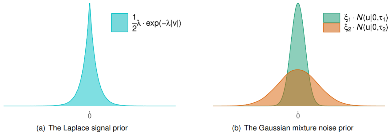
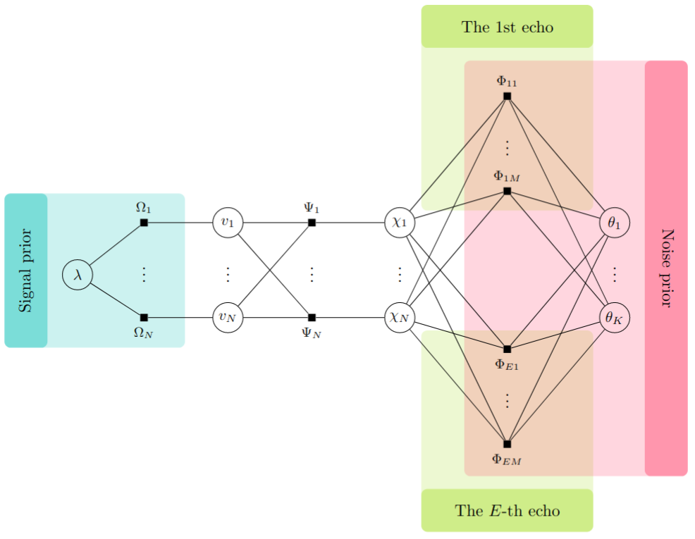
To deal with phase errors, we shall adopt the following nonlinear measurement model proposed by Liu et al. in [3]. At the $$$e$$$-th echo, we have$$\boldsymbol{W}_e \exp(i\boldsymbol\phi_e) = \boldsymbol{W}_e\exp(i\boldsymbol A_e\boldsymbol\chi)+\boldsymbol u$$where $$$\boldsymbol{W}_e$$$ is a diagonal weighting matrix, $$$\boldsymbol{A}_e$$$ is an operator that maps the susceptibility map $$$\boldsymbol \chi$$$ to the phase image $$$\boldsymbol \phi_e$$$, and $$$\boldsymbol u$$$ is the noise. As shown in Fig. 1(a), the wavelet coefficients $$$\boldsymbol v$$$ of the susceptibility $$$\boldsymbol\chi$$$ are assumed to follow the i.i.d. Laplace distribution:$$p(v|\lambda) = \frac{1}{2}\lambda\cdot\exp(-\lambda|v|)$$where $$$\lambda>0$$$ is the unknown distribution parameter. As shown in Fig. 1(b), we propose the following Gaussian-mixture distribution to model the long-tailed noise distribution$$p(u|\xi_s,\tau_s)=\sum_{s=1}^2\xi_s \cdot\mathcal{N}(u|0,\tau_s)$$where $$$\xi_s$$$ is the $$$s$$$-th mixture weight, $$$\tau_s$$$ is the $$$s$$$-th variance, the mixture means are zeros, and $$$\mathcal{N}(\cdot)$$$ is the Gaussian density function. The number of Gaussian mixtures needs to be chosen to avoid overfitting during reconstruction. From the experiments, we observed that two Gaussian mixtures produce the best performance. In particular, the variance $$$\tau_2$$$ of the second Gaussian component should be large enough to cover the domain of $$$u$$$, it is used to model the noise outliers that give rise to a long-tailed distribution. In practice, we can initialize the second variance $$$\tau_2$$$ with a larger value than the first variance $$$\tau_1$$$.Under the Bayesian formulation, we can recover $$$\boldsymbol\chi$$$ by computing its MAP estimation$$\widehat{\boldsymbol\chi} = \arg\max_{\boldsymbol\chi}\ p(\boldsymbol\chi|\boldsymbol y) $$where $$$\boldsymbol{y}$$$ contains the measurements, and $$$p(\boldsymbol\chi|\boldsymbol{y})$$$ is the posterior distribution of $$$\boldsymbol\chi$$$ that can be computed via approximate message passing (AMP) [4]. The factor graph of AMP is shown in Fig. 2.

Experimental Results

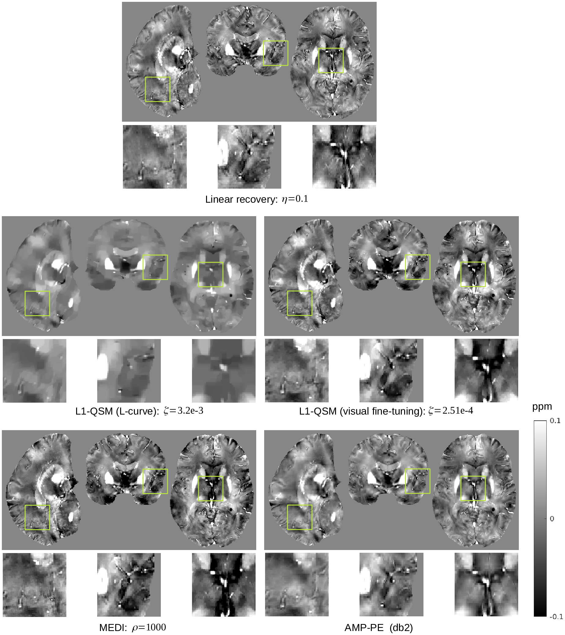
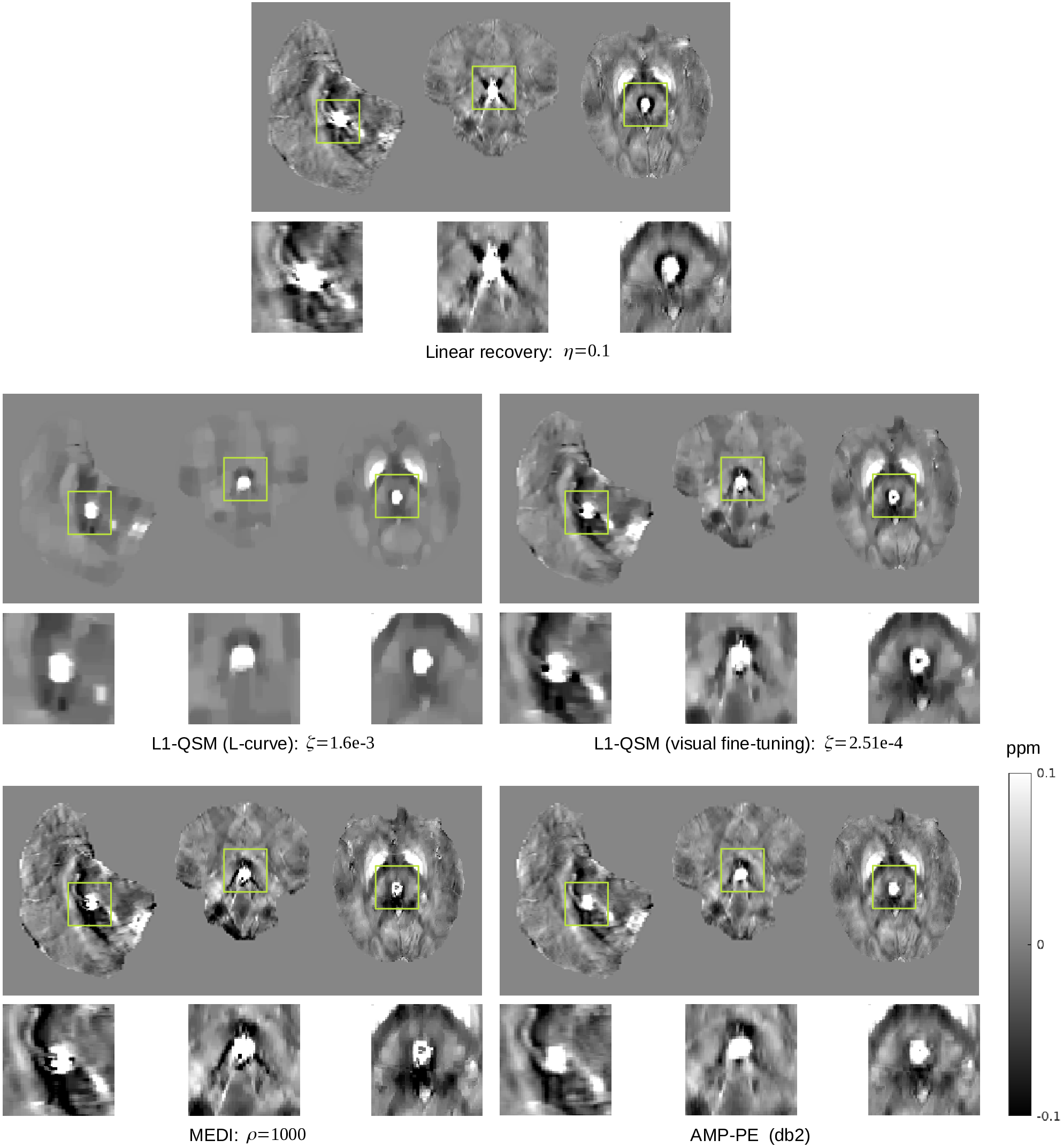
We compare the proposed AMP-PE approach with the linear recovery, the nonlinear L1-QSM [2] and MEDI [3] approaches on the in vivo 3D brain datasets acquired from healthy and (hemorrhage) patient scans. For the nonlinear L1-QSM approach, the parameters determined by the L-curve method over-regularized the reconstructions on the in vivo datasets, leading to the loss of finer details in recovered maps. As suggested in [2], we shall resort to visual fine-tuning to find working parameters for the nonlinear L1-QSM when the computed parameters fail. However, visual fine-tuning would introduce subjective bias to recovered susceptibility maps inevitably. For the MEDI approach, the default parameter $$$\rho=1000$$$ was used. In order to ensure MEDI achieves its best performance, we need to double check the results through visual fine-tuning as well. The recovered maps produced under the default parameter in MEDI were generally consistent with the visual fine-tuning results. For the linear recovery approach, the parameter $$$\eta=0.1$$$ was determined through visual fine-tuning. On the other hand, the proposed AMP-PE did not require visual fine-tuning since it estimated the parameters from the data automatically and adaptively. Fig. 3 and 4 show the recovered susceptibility maps from the healthy and patient scans respectively.

Discussion and Conclusion

For the healthy scan, the linear recovery and AMP-PE approaches were better than the nonlinear L1-QSM and MEDI at recovering the structural details. For the patient scan, AMP-PE revealed more structural details than the nonlinear L1-QSM and removed the streaking artifacts around the hemorrhage spot better than MEDI, indicating that the Gaussian-mixture noise prior is a better fit in this case. Additionally, the nonlinear L1-QSM and MEDI typically rely on visual fine-tuning to select or double-check working parameters for different MR protocols and scanners. The proposed AMP-PE is equipped with built-in parameter estimation, and could avoid subjective bias from the visual fine-tuning step, which makes it a better choice for the clinical setting.

Acknowledgements

This work is supported by National Institutes of Health under Grants R21AG064405, R01AG072603 and P30AG066511.