Synopsis

Keywords: Image Reconstruction, Brain

Head motion is accompanied by a multitude of second order motion effects like changing coil sensitivity maps, background field inhomogeneities, and susceptibility-induced fields. While scan geometries and shims can be corrected in real-time, the scanner has no means to counteract changes of the coil sensitivity maps or the susceptibility-induced fields requiring data-driven retrospective motion correction algorithms for these issues. Randomized sampling can further be exploited to improve the problem conditioning of the parameter estimations on temporal sub-segments of the scan. In this work, we evaluate the combination prospective motion navigation with randomized sampling in a pose-dependent field correction algorithm.

Introduction

In addition to rigid geometry mismatches, head motion is accompanied by a multitude of second order motion effects like changes in the coil sensitivity maps (CSM) [1], background field inhomogeneities, and susceptibility-induced fields [2]. While scan geometries [3] and shims [4] can be corrected in real-time, the scanner has no means to counteract changes of the CSM or the susceptibility-induced fields. The latter variations can, however, be addressed by data-driven retrospective motion correction algorithms [1,5,6]. Randomized sampling strategies (like DISORDER [7]) can further be exploited to spread the spatiotemporal sensing of the field changes evenly over the scan, improving the problem conditioning of the parameter estimations on temporal sub-segments of the scan [5]. In this work, we propose to combine prospective motion correction (PMC), implemented by a navigation approach [8,9], with randomized sampling for pose-dependent correction of field changes.

Theory

For rigid motion, the Sense model [10] needs to include the rigid coordinate transformation $$${\boldsymbol r}=T({\boldsymbol r^\prime},t)$$$ from scanner frame coordinates $$${\boldsymbol r^\prime}$$$ to head frame coordinates $$${\boldsymbol r}$$$ [11]. Assuming a perfect PMC without latencies, the influence of rigid motion on the k-space trajectory and the demodulation terms are already corrected. Thus, the signal $$$m_{\gamma}$$$ of coil $$${\gamma}$$$ can be written as:
$$m_{\gamma}({\boldsymbol k}(t))=\int\rho({\boldsymbol r})s_{\gamma}(T^{-1}({\boldsymbol r},t))e^{2\pi i T_E(d_x({\boldsymbol r})\theta_{x}(t)+d_y({\boldsymbol r})\theta_{y}(t))}e^{-i {\boldsymbol k}\cdot {\boldsymbol r}}d{\boldsymbol r},$$
with the signal density $$$\rho$$$, the $$$\gamma$$$-th CSM $$$s_{\gamma}$$$, the echo time $$$T_E$$$, and the k-space coordinate $$${\boldsymbol k}$$$. The linear coefficients (LC) maps $$$d_x({\boldsymbol r})$$$ and $$$d_y({\boldsymbol r})$$$ are used by Brackenier et al. [5] to approximate the susceptibility-induced field changes caused by the rotations $$$\theta_{x}(t)$$$ and $$$\theta_{y}(t)$$$ against the main field direction of the scanner. The LC maps and the signal density stay constant in the head frame coordinate $$${\boldsymbol r}$$$, while the CSM require inverse rigid rewarping [1].

Methods

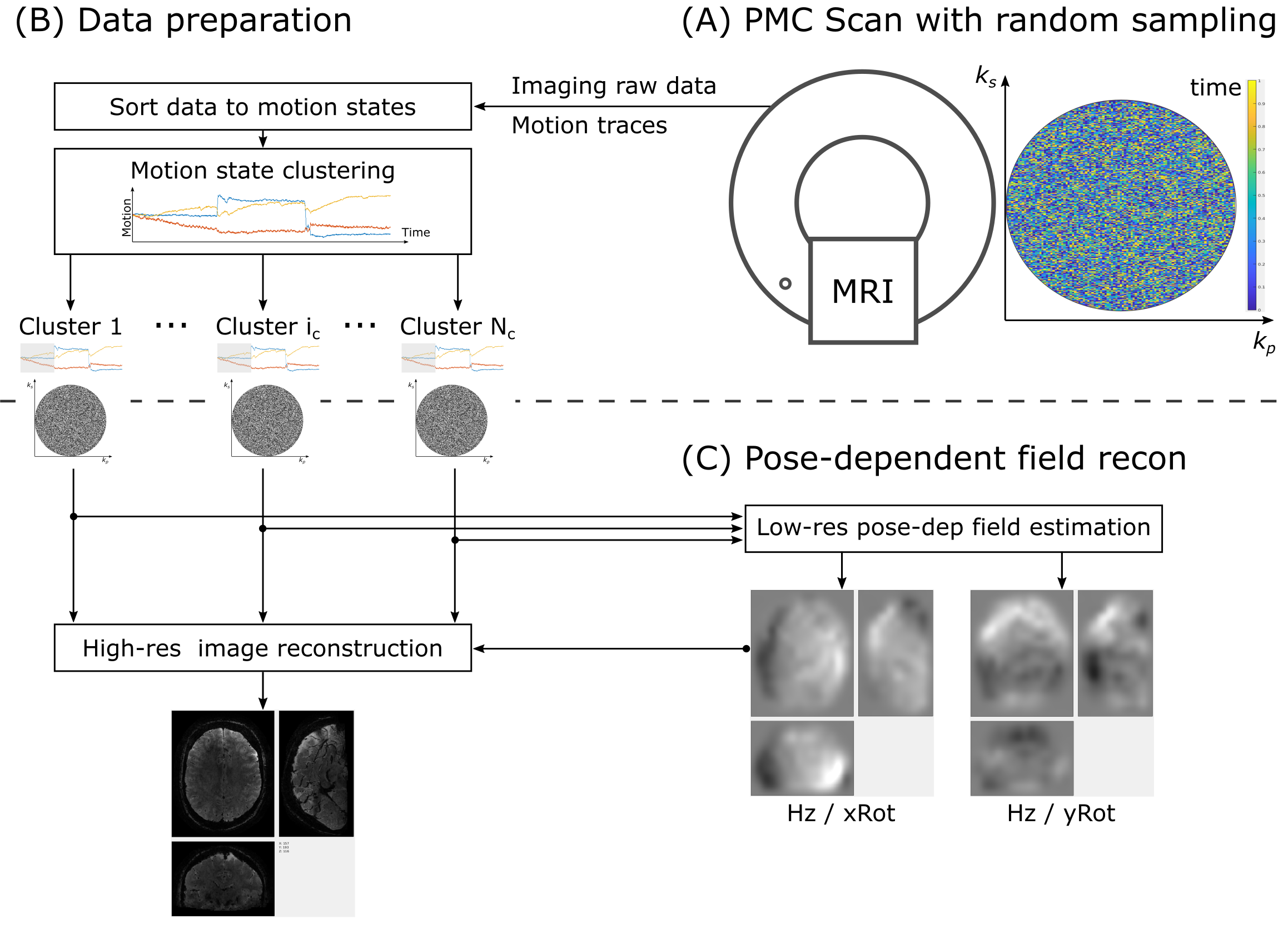
An overview of the image acquisition and reconstruction pipeline is shown in Fig. 1. Imaging data is acquired with a random acquisition pattern and a navigator-based PMC [8]. The imaging data and the motion traces are then fed into the reconstruction for motion state clustering. Next, the LC maps are calculated in the low-resolution pose-dependent field estimation and fed into the high-resolution image reconstruction.

The LC map $$$d_j({\boldsymbol r})$$$ were modeled in a 3D B-Spline basis $$$B$$$ with [20, 20, 10] knots in [x, y, z] directions to enforce smoothness and compress the number of parameters in the spline coefficient vector $$${\boldsymbol b}$$$ [12]:
$$d_j({\boldsymbol r})=B{\boldsymbol b}_j,\quad j=\{x, y\}.$$

The optimization problem can be written as a sum over the data discrepancies of the $$$N_c$$$ clusters:
$$(\hat{\boldsymbol \rho},\hat{\boldsymbol b}_{x},\hat{\boldsymbol b}_{y})=\underset{({\boldsymbol \rho}, {\boldsymbol b}_{x},{\boldsymbol b}_{y})}{\text{argmin}}\sum_{c=1}^{N_c}\lVert M_cFS_c({\boldsymbol \rho}\circ e^{2\pi iT_E(B\cdot{\boldsymbol b}_{x}\theta_{x,c}+B\cdot{\boldsymbol b}_{y}\theta_{y,c})})-{\boldsymbol m}_c\rVert_2^2,$$
where $$$\theta_{x,c}$$$ denominates the averaged cluster rotation around X. $$$M_c$$$, $$$F$$$ and $$$S_c$$$ are the masking, Fourier and Sense operators. The minimization is solved by alternating optimization between $$$\hat{\boldsymbol \rho}$$$ and $$$(\hat{\boldsymbol b}_{x}, \hat{\boldsymbol b}_{y})$$$ using the conjugate gradient method for $$$\hat{\boldsymbol \rho}$$$ and gradient descent optimization for $$$(\hat{\boldsymbol b}_{x}, \hat{\boldsymbol b}_{y})$$$. The calculation of the gradients with respect to the LC-induced phase maps follows the descriptions of Refs. [5,13]. The gradient descent uses a backtracking line search and was implemented on halved resolution. At most 20 alternating cycles were performed, where each cycle contains one image reconstruction and 10 gradient descent updates for the spline coefficients.

The scans were performed on a 7T Philips Achieva Scanner (Best, The Netherlands) with a 32-channel coil. A navigated 3D GRE imaging sequence was used [8] for multi-echo scans with two contrasts at 0.6 x 0.6 x 1.2 mm^3 resolution. The first contrast had $$$T_E=\{8.1,12.1,16.1\}ms$$$, $$$T_R=20ms$$$, $$$FA=3°$$$, 9:30 min. The second contrast had $$$T_E=\{7.7, 16.3, 24.8\}ms$$$, $$$T_R=42ms$$$, $$$FA=18°$$$, 19:00 min.

Two subjects were scanned once without instructed motion and once repeating a motion pattern, where the head was rotated in the order [$$$+\theta_x$$$, $$$-\theta_x$$$, $$$+\theta_y$$$, $$$-\theta_y$$$] after every fifth of the scan time. The proposed method was compared to a motion-adapted Sense algorithm, which solves the optimization in Eq. 3 once by CG with warped coil sensitivity maps but no LC field maps.

Results

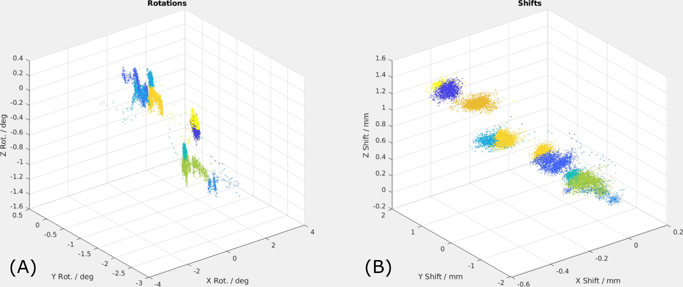
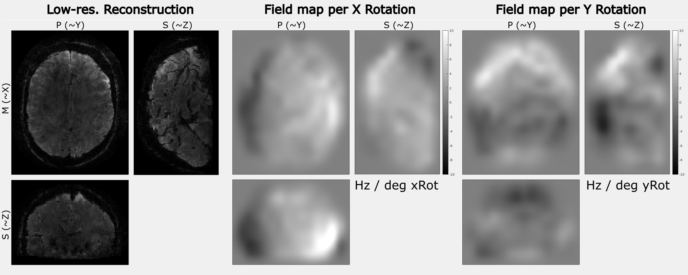
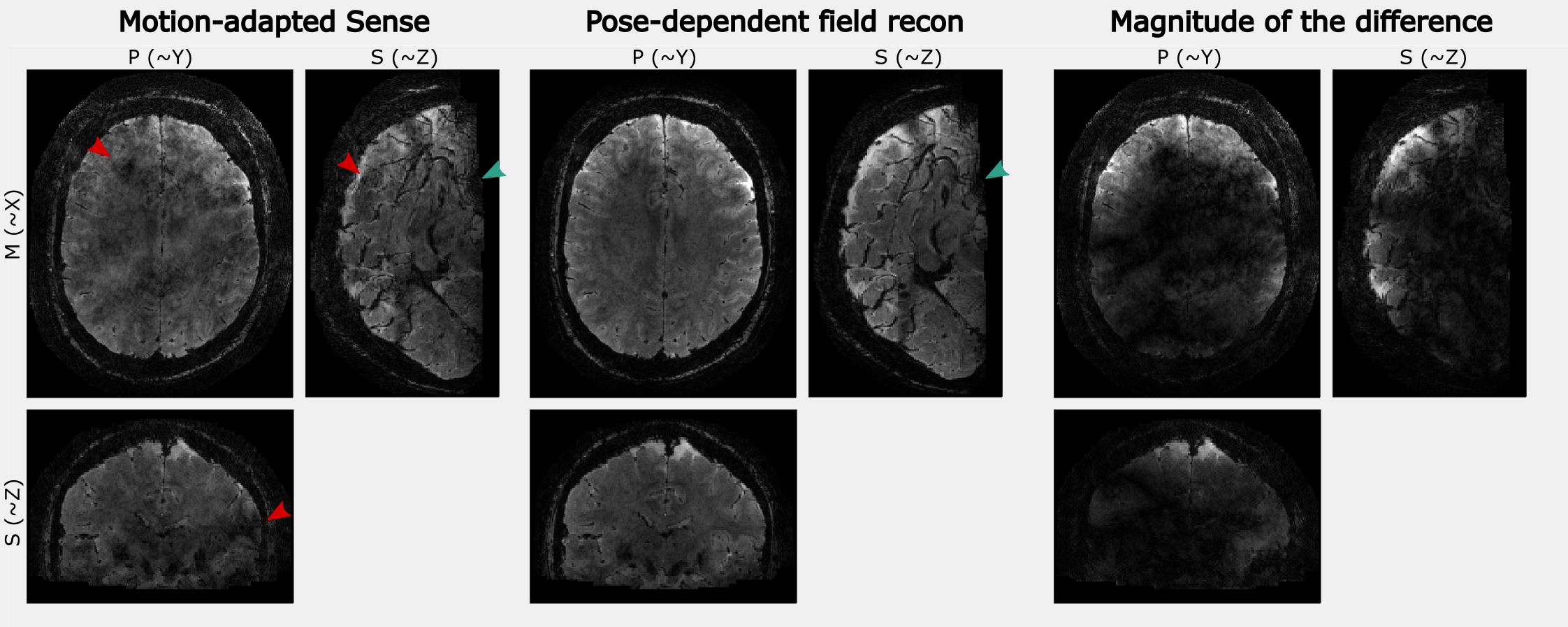
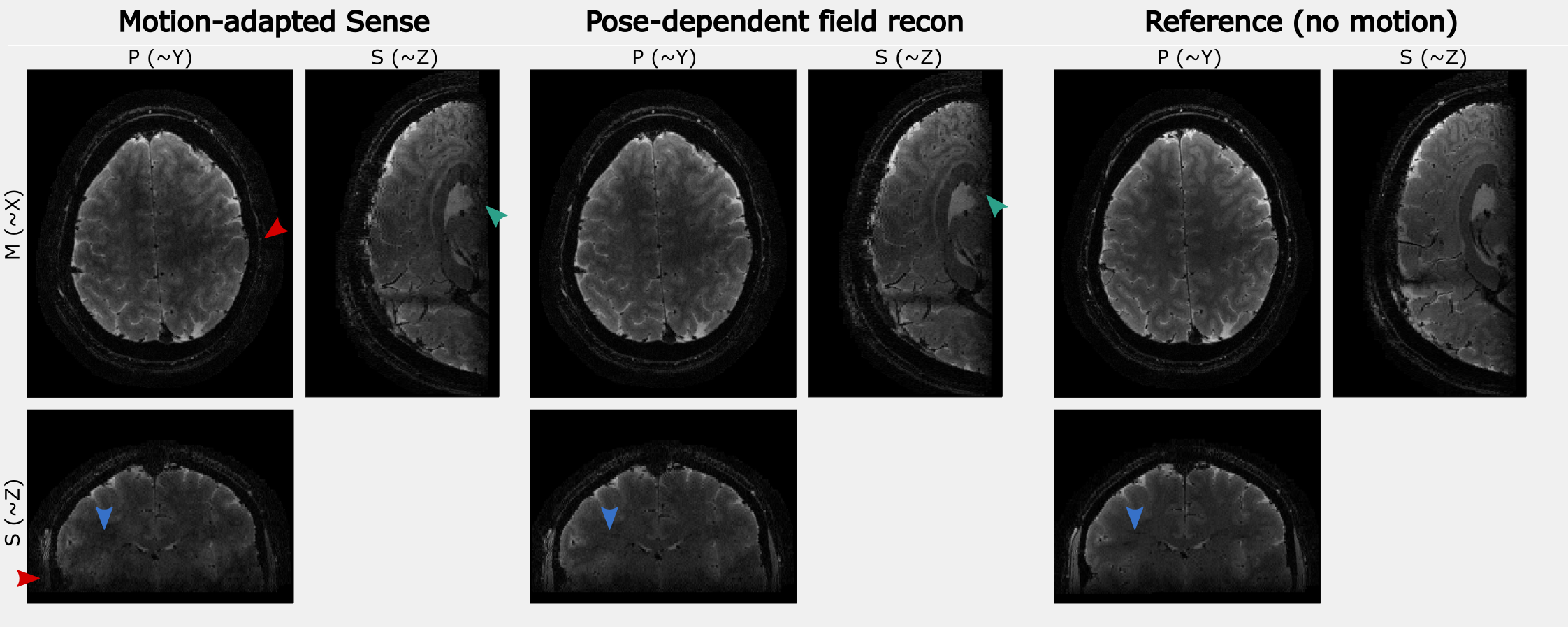
Figures 2-4 show the results of one in-vivo dataset ($$$T_E=24.8ms$$$) for the motion clustering, pose-dependent field estimation and the high-resolution image reconstruction, respectively. The LC maps range from $$$[-10,10]Hz$$$ for motion parameters of $$$[-1.5,1.5]mm$$$ and $$$[-3, 2]deg$$$. The image artifacts of motion-adapted Sense in Fig. 4 were clearly reduced by the proposed method.
Figure 5 compares the high-resolution image reconstruction results ($$$T_E=16.1ms$$$) of the second subject to the motion-adapted Sense and a reference scan without motion. The estimated fields were in the range of $$$[-20,20]Hz$$$ for motion parameters of $$$[-1,1]mm$$$ and $$$[-1,1]deg$$$.

Discussion and conclusion

The proposed method produces parameter-dependent field maps that are consistent with previous descriptions of motion-induced fields [2]. The inclusion of the field maps in the image reconstruction tremendously improves image quality. The combination of retrospective 2nd order motion corrections with prospective corrections reduces the computational load on the reconstruction side, reduces Nyquist ghosting artifacts, and considerably improves the starting conditions for such demanding non-convex algorithms. By this, we were able to reconstruct datasets with TEs of up to 25 ms.

Acknowledgements

This work has received funding from the European Union’s Horizon 2020 research and innovation program under grant agreement No. 885876 (AROMA project).